
Computing laminar and turbulent moisture flows in air is both flexible and user friendly with the Moisture Flow multiphysics interfaces and coupling in the COMSOL Multiphysics® software. Available as of version 5.3a, this comprehensive set of functionality can be used to model coupled heat and moisture transport in air and building materials. Let’s learn how the Moisture Flow interface complements existing functionality, while highlighting its benefits.
Modeling Heat and Moisture Transport
Modeling the transport of heat and moisture through porous materials, or from the surface of a fluid, often involves including the surrounding media in the model in order to get accurate estimates of the conditions at the material surfaces. In the investigations of hygrothermal behavior of building envelopes, food packaging, and other common engineering problems, the surrounding medium is probably moist air (air with water vapor).
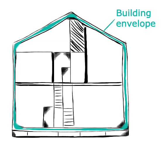
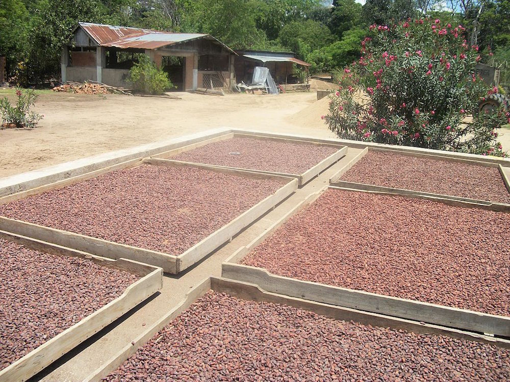
Moist air is the environing medium for applications such as building envelopes (illustration, left) and solar food drying (right). Right image by ArianeCCM — Own work. Licensed under CC BY-SA 3.0, via Wikimedia Commons.
When considering porous media, the moisture transport process, which includes capillary flow, bulk flow, and binary diffusion of water vapor in air, depends on the nature of the material. In moist air, moisture is transported by diffusion and advection, where the advecting flow field in most cases is turbulent.
Computing heat and moisture transport in moist air requires the resolution of three sets of equations:
- The Navier-Stokes equations, to compute the airflow velocity field \mathbf{u} and pressure p
- The energy equation, to compute the temperature T
- The moisture transport equation, to compute the relative humidity \phi
These equations are coupled together through the pressure, temperature, and relative humidity, which are used to evaluate the properties of air (density \rho(p,T,\phi); viscosity \mu(T,\phi); thermal conductivity k(T,\phi); and heat capacity C_p(T,\phi)); molecular diffusivity D(T) and through the velocity field used for convective transport.
With the addition of the Moisture Flow multiphysics interface in version 5.3a, COMSOL Multiphysics defines all three of these equations in a few steps, as shown in the figure below.

Single-physics interfaces and multiphysics couplings for the coupled resolution of single-phase flow, heat transfer, and moisture transport in building materials and moist air.
Using the Moisture Flow Multiphysics Interface
Whenever studying the flow of moist air, two questions should be asked:
- Does the flow depend on moisture distribution?
- Does the nature of the flow require the use of a turbulence model?
If the answer is “yes” for at least one of these questions, then you should consider using the Moisture Flow multiphysics interfaces, found under the Chemical Species Transport branch.

The Moisture Flow group under the Chemical Species Transport branch of the Physics Wizard, with the single-physics interfaces and coupling node added with each version of the Moisture Flow predefined multiphysics interface.
The Laminar Flow version of the multiphysics interface combines the Moisture Transport in Air interface with the Laminar Flow interface and adds the Moisture Flow coupling. Similarly, each version under Turbulent Flow combines the Moisture Transport in Air interface and the corresponding Turbulent Flow interface and adds the Moisture Flow coupling.
Besides providing a user-friendly way to define the coupled set of equations of the moisture flow problem, the multiphysics interfaces for turbulent flow handle the moisture-related turbulence variables required for the fluid flow computation.
Automatic Coupling Between Single-Physics Interfaces
One advantage of using the Moisture Flow multiphysics interface is its usability. When adding the Moisture Flow node through the predefined interface, an automatic coupling of the Navier-Stokes equations is defined for the fluid flow and the moisture transport equations by the software (center screenshot in the image below) by using the following variables:
- The density and dynamic viscosity in the Navier-Stokes equations, which depend on the relative humidity variable from the Moisture Transport interface through a mixture formula based on dry air and pure steam properties (left screenshot below)
- The velocity field and absolute pressure variables from the Single-Phase Flow interface, which are used in the moisture transport equation (right screenshot below)

User interfaces of the Moisture Flow coupling, Fluid Properties feature (Single-Phase Flow interface), and Moist Air feature (Moisture Transport in Air interface).
Support for Turbulent Fluid Flow
The performance of the Moisture Flow multiphysics interface is especially attractive when dealing with a turbulent moisture flow.
For turbulent flows, the turbulent mixing caused by the eddy diffusivity in the moisture convection is automatically accounted for by the COMSOL® software by enhancing the moisture diffusivity with a correction term based on the turbulent Schmidt number . The Kays-Crawford model is the default choice for the evaluation of the turbulent Schmidt number, but a user-defined value or expression can also be entered directly in the graphical user interface.
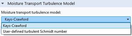
Selection of the model for the computation of the turbulent Schmidt number in the user interface of the Moisture Flow coupling.
In addition, for coarse meshes that may not be suitable for resolving the thin boundary layer close to walls, Wall functions can be selected or automatically applied by the software. The wall functions are such that the computational domain is assumed to be located at a distance from the wall, the so-called lift-off position, corresponding to the distance from the wall where the logarithmic layer meets the viscous sublayer (or would meet it if there was no buffer layer in between). The moisture flux at the lift-off position, g_{wf}, which accounts for the flux to and from the wall, is automatically defined by the Moisture Flow interface, based on the relative humidity.
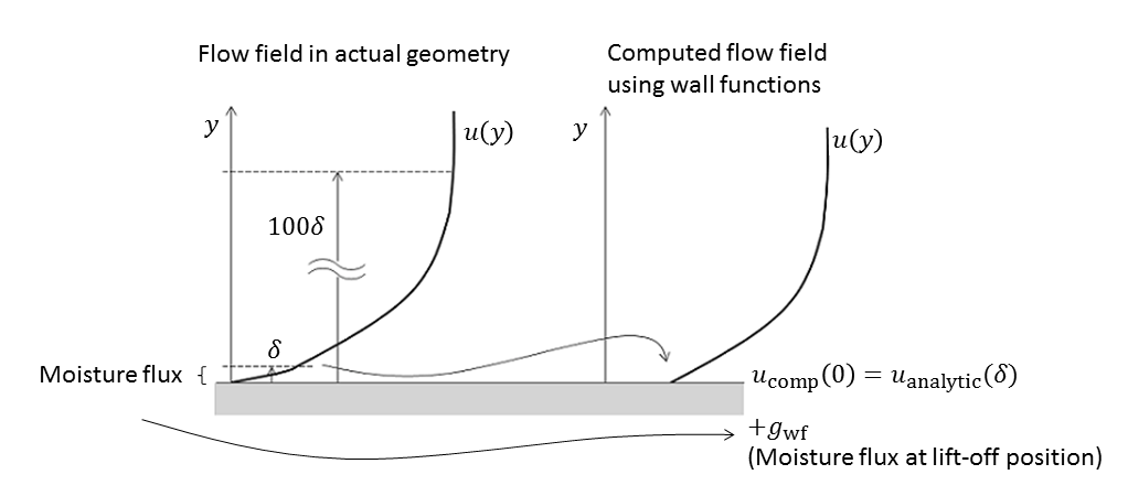
Approximation of the flow field and the moisture flux close to walls when using wall functions in the turbulence model for fluid flow.
Note that the Low-Reynolds and Automatic options for Wall Treatment are also available for some of the RANS models.
For more information, read this blog post on choosing a turbulence model.
Mass Conservation Across Boundaries
By using the Moisture Flow interface, an appropriate mass conservation is granted in the fluid flow problem by the Screen and Interior Fan boundary conditions. A continuity condition is also applied on vapor concentration at the boundaries where the Screen feature is applied. For the Interior Fan condition, the mass flow rate is conserved in an averaged way and the vapor concentration is homogenized at the fan outlet, as shown in the figure below.
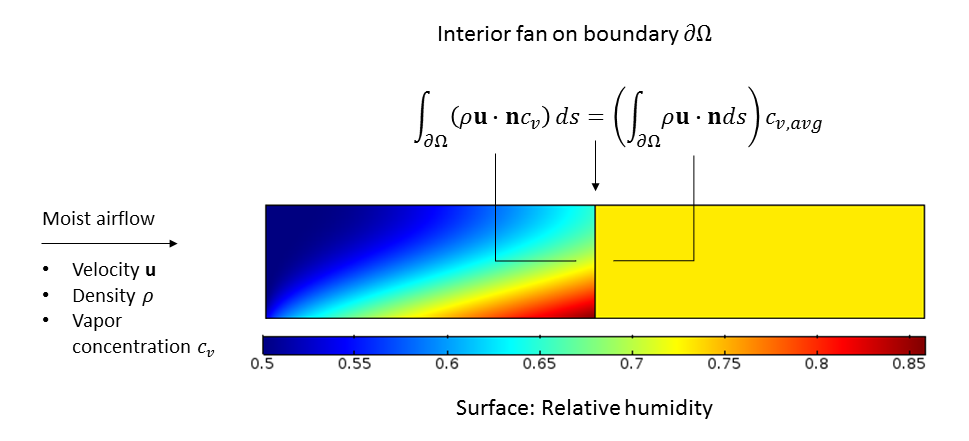
Average mass flow rate conservation across a boundary with the Interior Fan condition.
Example: Modeling Evaporative Cooling with the Moisture Flow Interface
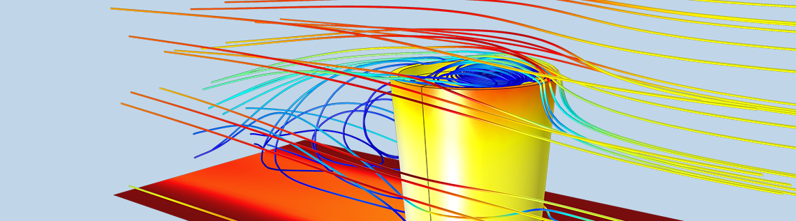
Let’s consider evaporative cooling at the water surface of a glass of water placed in a turbulent airflow. The Turbulent Flow, Low Reynolds k-ε interface, the Moisture Transport in Air interface, and the Heat Transfer in Moist Air interface are coupled through the Nonisothermal Flow, Moisture Flow, and Heat and Moisture coupling nodes. These couplings compute the nonisothermal airflow passing over the glass, the evaporation from the water surface with the associated latent heat effect, and the transport of both heat and moisture away from this surface.
By using the Automatic option for Wall treatment in the Turbulent Flow, Low Reynolds k-ε interface, wall functions are used if the mesh resolution is not fine enough to fully resolve the velocity boundary layer close to the walls. Convective heat and moisture fluxes at lift-off position are added by the Nonisothermal Flow and Moisture Flow couplings. The temperature and relative humidity solutions after 20 minutes are shown below, along with the streamlines of the airflow velocity field.


Temperature (left) and relative humidity (right) solutions with the streamlines of the velocity field after 20 minutes.
The temperature and relative humidity fields have a strong resemblance here, which is quite natural since the fields are strongly coupled and since both transport processes have similar boundary conditions, in this case. In addition, heat transfer is given by conduction and advection while mass transfer is described by diffusion and advection. The two transport processes originate from the same physical phenomena: conduction and diffusion from molecular interactions in the gas phase while advection is given by the total motion of the bulk of the fluid. Also, the contribution of the eddy diffusivity to the turbulent thermal conductivity and the turbulent diffusivity originate from the same physical phenomenon, which adds further to the similarity of the temperature and moisture field.
Next Steps
Learn more about the key features and functionality included with the Heat Transfer Module, and add-on to COMSOL Multiphysics:
Read the following blog posts to learn more about heat and moisture transport modeling:
- How to Model Heat and Moisture Transport in Porous Media with COMSOL®
- How to Model Heat and Moisture Transport in Air with COMSOL®
Get a demonstration of the Nonisothermal Flow and Heat and Moisture couplings in these tutorial models:


Comments (3)
Ugur ACAR
February 22, 2019Hi,
Let me briefly explain closed circuit cooling towers first. Air is drawn into the tower from the bottom leaves through the top flowing on and around the cooling coil while water is sprayed on the cooling coil. Water which is desired to be cooled circulates in the cooling coil consist of tubes. It is assumed that a thin film layer of water occurs at outer sides of cooling coil tubes. As thin water layer evaporatively cooled due to air flow, water which circulates in the coil cooled at the same time. I was wondering if is it possible to simulate heat and mass transfer mechanism for closed circuit wet cooling towers. is Comsol enough to do that or any experimental data needed?
thank you.
Claire Bost
February 22, 2019 COMSOL EmployeeHi Ugur,
the Moisture Transport interface can be used to model the evaporation occuring at the outer surface of the cooling coil, and the transport of vapor in the moist air flow. The only limitation I see is for the modeling of droplets, which seem to be present if I understand well your description. Indeed, the Moisture Transport interface is valid in moist air, where only air and vapor are present. Maybe in this application the transport of droplets may be neglected?
For the evaporation on thin film layer, the Moist Surface boundary condition can be used.
Best Regards,
Claire
Waseem Raza
March 29, 2022Hi Claire Bost,
Could you please guide me on how to model and simulate moisture transport on a wall surface? or any other helping material.