
The COMSOL Multiphysics® software offers several different formulations for solving turbulent flow problems: the L-VEL, algebraic yPlus, Spalart-Allmaras, k-ε, k-ω, low Reynolds number k-ε, SST, and v2-f turbulence models. These formulations are available in the CFD Module, and the L-VEL, algebraic yPlus, k-ε, and low Reynolds number k-ε models are also available in the Heat Transfer Module. In this blog post, learn why to use these various turbulence models, how to choose between them, and how to use them efficiently.
This post was originally published in 2013. It has since been updated to include all of the turbulence models currently available with the CFD Module as of version 5.3 of the COMSOL® software.
Introduction to Turbulence Modeling
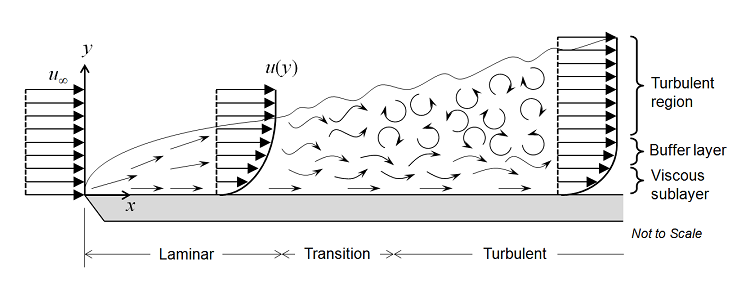
Let’s start by considering the fluid flow over a flat plate, as shown in the figure below. The uniform velocity profile hits the leading edge of the flat plate, and a laminar boundary layer begins to develop. The flow in this region is very predictable. After some distance, small chaotic oscillations begin to develop in the boundary layer and the flow begins to transition to turbulence, eventually becoming fully turbulent.
The transition between these three regions can be defined in terms of the Reynolds number, Re=\rho v L/\mu, where \rho is the fluid density; v is the velocity; L is the characteristic length (in this case, the distance from the leading edge); and \mu is the fluid’s dynamic viscosity. We will assume that the fluid is Newtonian, meaning that the viscous stress is directly proportional, with the dynamic viscosity as the constant of proportionality, to the shear rate. This is true, or very nearly so, for a wide range of fluids of engineering importance, such as air or water. Density can vary with respect to pressure, although it is here assumed that the fluid is only weakly compressible, meaning that the Mach number is less than about 0.3. The weakly compressible flow option for the fluid flow interfaces in COMSOL Multiphysics neglects the influence of pressure waves on the flow and pressure fields.
In the laminar regime, the fluid flow can be completely predicted by solving Navier-Stokes equations, which gives the velocity and the pressure fields. Let us first assume that the velocity field does not vary with time. An example of this is outlined in The Blasius Boundary Layer tutorial model. As the flow begins to transition to turbulence, oscillations appear in the flow, despite the fact that the inlet flow rate does not vary with time. It is then no longer possible to assume that the flow is invariant with time. In this case, it is necessary to solve the time-dependent Navier-Stokes equations, and the mesh used must be fine enough to resolve the size of the smallest eddies in the flow. Such a situation is demonstrated in the Flow Past a Cylinder tutorial model. Note that the flow is unsteady, but still laminar in this model. Steady-state and time-dependent laminar flow problems do not require any modules and can be solved with COMSOL Multiphysics alone.

As the flow rate — and thus also the Reynolds number — increases, the flow field exhibits small eddies and the spatial and temporal scales of the oscillations become so small that it is computationally unfeasible to resolve them using the Navier-Stokes equations, at least for most practical cases. In this flow regime, we can use a Reynolds-averaged Navier-Stokes (RANS) formulation, which is based on the observation that the flow field (u) over time contains small, local oscillations (u’) and can be treated in a time-averaged sense (U). For one- and two-equation models, additional transport equations are introduced for turbulence variables, such as the turbulence kinetic energy (k in k-ε and k-ω).
In algebraic models, algebraic equations that depend on the velocity field — and, in some cases, on the distance from the walls — are introduced in order to describe the turbulence intensity. From the estimates for the turbulence variables, an eddy viscosity that adds to the molecular viscosity of the fluid is calculated. The momentum that would be transferred by the small eddies is instead translated to a viscous transport. Turbulence dissipation usually dominates over viscous dissipation everywhere, except for in the viscous sublayer close to solid walls. Here, the turbulence model has to continuously reduce the turbulence level, such as in low Reynolds number models. Or, new boundary conditions have to be computed using wall functions.
Low Reynolds Number Models
The term “low Reynolds number model” sounds like a contradiction, since flows can only be turbulent if the Reynolds number is high enough. The notation “low Reynolds number” does not refer to the flow on a global scale, but to the region close to the wall where viscous effects dominate; i.e., the viscous sublayer in the figure above. A low Reynolds number model is a model that correctly reproduces the limiting behaviors of various flow quantities as the distance to the wall approaches zero. So, a low Reynolds number model must, for example, predict that k~y2 as y→0. Correct limiting behavior means that the turbulence model can be used to model the whole boundary layer, including the viscous sublayer and the buffer layer.
Most ω-based models are low Reynolds number models by construction. But the standard k-ε model and other commonly encountered k-ε models are not low Reynolds number models. Some of them can, however, be supplemented with so-called damping functions that give the correct limiting behavior. They are then known as low Reynolds number k-ε models.
Low Reynolds number models often give a very accurate description of the boundary layer. The sharp gradients close to walls do, however, require very high mesh resolutions and that, in turn, means that the high accuracy comes at a high computational cost. This is why alternative methods to model the flow close to walls are often employed for industrial applications.
Wall Functions
The turbulent flow near a flat wall can be divided into four regions. At the wall, the fluid velocity is zero, and in a thin layer above this, the flow velocity is linear with distance from the wall. This region is called the viscous sublayer, or laminar sublayer. Further away from the wall is a region called the buffer layer. In the buffer region, turbulence stresses begin to dominate over viscous stresses and it eventually connects to a region where the flow is fully turbulent and the average flow velocity is related to the log of the distance to the wall. This is known as the log-law region. Even further away from the wall, the flow transitions to the free-stream region. The viscous and buffer layers are very thin and if the distance to the end of the buffer layer is \delta, then the log-law region will extend about 100\delta away from the wall.

It is possible to use a RANS model to compute the flow field in all four of these regions. However, since the thickness of the buffer layer is so small, it can be advantageous to use an approximation in this region. Wall functions ignore the flow field in the buffer region and analytically compute a nonzero fluid velocity at the wall. By using a wall function formulation, you assume an analytic solution for the flow in the viscous layer and the resultant models will have significantly lower computational requirements. This is a very useful approach for many practical engineering applications.

If you need a level of accuracy beyond what the wall function formulations provide, then you will want to consider a turbulence model that solves the entire flow regime as described for the low Reynolds number models above. For example, you may want to compute lift and drag on an object or compute the heat transfer between the fluid and the wall.
Automatic Wall Treatment
The automatic wall treatment functionality, which is new in COMSOL Multiphysics version 5.3, combines benefits from both wall functions and low Reynolds number models. Automatic wall treatment adapts the formulation to the mesh available in the model so that you get both robustness and accuracy. For instance, for a coarse boundary layer mesh, the feature will utilize a robust wall function formulation. However, for a dense boundary layer mesh, the automatic wall treatment will use a low Reynolds number formulation to resolve the velocity profile completely to the wall.
Going from a low Reynolds number formulation to a wall function formulation is a smooth transition. The software blends the two formulations in the boundary elements. Then, the software calculates the wall distance of the boundary elements’ grid points (this is in viscous units given by a liftoff). The combined formulations are then used for the boundary conditions.
All turbulence models in COMSOL Multiphysics, except the k-ε model, support automatic wall treatment. This means that the low Reynolds number models can be used for industrial applications and that their low Reynolds number modeling capability is only invoked when the mesh is fine enough.
About the Various Turbulence Models
The eight RANS turbulence models differ in how they model the flow close to walls, the number of additional variables solved for, and what these variables represent. All of these models augment the Navier-Stokes equations with an additional turbulence eddy viscosity term, but they differ in how it is computed.
L-VEL and yPlus
The L-VEL and algebraic yPlus turbulence models compute the eddy viscosity using algebraic expressions based only on the local fluid velocity and the distance to the closest wall. They do not solve any additional transport equations. These models solve for the flow everywhere and are the most robust and least computationally intensive of the eight turbulence models. While they are generally the least accurate models, they do provide good approximations for internal flow, especially in electronic cooling applications.
Spalart-Allmaras
The Spalart-Allmaras model adds a single additional variable for an undamped kinematic eddy viscosity. It is a low Reynolds number model and can resolve the entire flow field down to the solid wall. The model was originally developed for aerodynamics applications and is advantageous in that it is relatively robust and has moderate resolution requirements. Experience shows that this model does not accurately compute fields that exhibit shear flow, separated flow, or decaying turbulence. Its advantage is that it is quite stable and shows good convergence.
k-ε
The k-ε model solves for two variables: k, the turbulence kinetic energy; and ε (epsilon), the rate of dissipation of turbulence kinetic energy. Wall functions are used in this model, so the flow in the buffer region is not simulated. The k-ε model has historically been very popular for industrial applications due to its good convergence rate and relatively low memory requirements. It does not very accurately compute flow fields that exhibit adverse pressure gradients, strong curvature to the flow, or jet flow. It does perform well for external flow problems around complex geometries. For example, the k-ε model can be used to solve for the airflow around a bluff body.
The turbulence models listed below are all more nonlinear than the k-ε model and they can often be difficult to converge unless a good initial guess is provided. The k-ε model can be used to provide a good initial guess. Just solve the model using the k-ε model and then use the Generate New Turbulence Interface functionality. Learn more about this functionality in the last part of the second video in this Learning Center article.
k-ω
The k-ω model is similar to the k-ε model, but it solves for ω (omega) — the specific rate of dissipation of kinetic energy. It is a low Reynolds number model, but it can also be used in conjunction with wall functions. It is more nonlinear, and thereby more difficult to converge than the k-ε model, and it is quite sensitive to the initial guess of the solution. The k-ω model is useful in many cases where the k-ε model is not accurate, such as internal flows, flows that exhibit strong curvature, separated flows, and jets. A good example of internal flow is flow through a pipe bend.
Low Reynolds Number k-ε
The low Reynolds number k-ε model is similar to the k-ε model, but does not need wall functions: it can solve for the flow everywhere. It is a logical extension of the k-ε model and shares many of its advantages, but generally requires a denser mesh; not only at walls, but everywhere its low Reynolds number properties kick in and dampen the turbulence. It can sometimes be useful to use the k-ε model to first compute a good initial condition for solving the low Reynolds number k-ε model. An alternative way is to use the automatic wall treatment and start with a coarse boundary layer mesh to get wall functions and then refine the boundary layer at the interesting walls to get the low Reynolds number models.
The low Reynolds number k-ε model can compute lift and drag forces and heat fluxes can be modeled with higher accuracy compared to the k-ε model. It has also shown to predict separation and reattachment quite well for a number of cases.
SST
The SST model is a combination of the k-ε model in the free stream and the k-ω model near the walls. It is a low Reynolds number model and kind of the “go to” model for industrial applications. It has similar resolution requirements to the k-ω model and the low Reynolds number k-ε model, but its formulation eliminates some weaknesses displayed by pure k-ω and k-ε models. In a tutorial model example, the SST model solves for flow over a NACA 0012 Airfoil. The results are shown to compare well with experimental data.
v2-f
Close to wall boundaries, the fluctuations of the velocity are usually much larger in the parallel directions to the wall in comparison with the direction perpendicular to the wall. The velocity fluctuations are said to be anisotropic. Further away from the wall, the fluctuations are of the same magnitude in all directions. The velocity fluctuations become isotropic.
The v2-f turbulence model describes the anisotropy of the turbulence intensity in the turbulent boundary layer using two new equations, in addition to the two equations for turbulence kinetic energy (k) and dissipation rate (ε). The first equation describes the transport of turbulent velocity fluctuations normal to the streamlines. The second equation accounts for nonlocal effects such as the wall-induced damping of the redistribution of turbulence kinetic energy between the normal and parallel directions.
You should use this model for enclosed flows over curved surfaces, for example, to model cyclones.
Meshing Considerations for CFD Problems
Solving for any kind of fluid flow problem — laminar or turbulent — is computationally intensive. Relatively fine meshes are required and there are many variables to solve for. Ideally, you would have a very fast computer with many gigabytes of RAM to solve such problems, but simulations can still take hours or days for larger 3D models. Therefore, we want to use as simple a mesh as possible, while still capturing all of the details of the flow.
Referring back to the figure at the top of this blog post, we can observe that for the flat plate (and for most flow problems), the velocity field changes quite slowly in the direction tangential to the wall, but quite rapidly in the normal direction, especially if we consider the buffer layer region. This observation motivates the use of a boundary layer mesh. Boundary layer meshes (which are the default mesh type on walls when using our physics-based meshing) insert thin rectangles in 2D or triangular prisms in 3D at the walls. These high-aspect-ratio elements will do a good job of resolving the variations in the flow speed normal to the boundary, while reducing the number of calculation points in the direction tangential to the boundary.

The boundary layer mesh (magenta) around an airfoil and the surrounding triangular mesh (cyan) for a 2D mesh.

The boundary layer mesh (magenta) around a bluff body and the surrounding tetrahedral mesh (cyan) for a 3D volumetric mesh.
Evaluating the Results of Your Turbulence Model
Once you’ve used one of these turbulence models to solve your flow simulation, you will want to verify that the solution is accurate. Of course, as you do with any finite element model, you can simply run it with finer and finer meshes and observe how the solution changes with increasing mesh refinement. Once the solution does not change to within a value you find acceptable, your simulation can be considered converged with respect to the mesh. However, there are additional values you need to check when modeling turbulence.
When using wall function formulations, you will want to check the wall resolution viscous units (this plot is generated by default). This value tells you how far into the boundary layer your computational domain starts and should not be too large. You should consider refining your mesh in the wall normal direction if there are regions where the wall resolution exceeds several hundred. The second variable that you should check when using wall functions is the wall liftoff (in length units). This variable is related to the assumed thickness of the viscous layer and should be small relative to the surrounding dimensions of the geometry. If it is not, then you should refine the mesh in these regions as well.

The maximum wall liftoff in viscous units is less than 100, so there is no need to refine the boundary layer mesh.
When solving a model using low Reynolds number wall treatment, check the dimensionless distance to cell center (also generated by default). This value should be of order unity everywhere for the algebraic models and less than 0.5 for all two-equation models and the v2-f model. If it is not, then refine the mesh in these regions.
Concluding Thoughts
In this blog post, we have discussed the various turbulence models available in COMSOL Multiphysics, highlighting when and why you should use each one of them. The real strength of the COMSOL® software is when you want to combine your fluid flow simulations with other physics, such as finding stresses on a solar panel in high winds, forced convection modeling in a heat exchanger, or mass transfer in a mixer, among other possibilities.
If you are interested in using the COMSOL® software for your CFD and multiphysics simulations, or if you have a question that isn’t addressed here, please contact us.


Comments (15)
Nagi Elabbasi
September 18, 2013That was very informative, thank you. Modeling turbulence accurately is not easy, so it’s good to see the COMSOL features and capabilities available for that purpose.
Franco Cerna
October 5, 2013Someone could hang a video tutorial on turbulent flows?
Mustafa Abd El-Mageed
November 9, 2013Can we use turbulent model type in FSI Physics in comsol 4.2a ? as the turbulent model consider the solid domain belong to the fluid and makes error message
Failed to evaluate variable.
– Variable: mod1.epx
– Geometry: 1
– Domain: 2 3 4 5
and all domains 2 3 4 5 are solids ?
Zaid B. Jildeh
December 2, 2014Thank you, this post helped me a lot to understand the nature of my system.
Thank to Comsol for updating the turbulent models, the new models in v.5.0 are very stable and fast to solve time-dependent response.
Angelo Fonseca
January 25, 2017How can you determine if the boundary layer mesh has the correct total thickness to resolve all the velocity profile from the no-slip wall to the freestream velocity?
Walter Frei
February 2, 2017 COMSOL EmployeeHello Angelo,
I believe that what you’re asking about here is a mesh refinement study:
https://www.comsol.com/multiphysics/mesh-refinement
Rami Hosseini
November 16, 2017Hello Walter thanks for your helpful topics.
I want to simulate lightning induced voltages on power systems by Comsol can you guide me that how can i do that?
Abdelrahman Hussain
December 2, 2017Thanks Walter for the nice illustration.
I want to analyze a flow in a geometry exactly the same as one shown in the last figure that shows the wall lift-off in a viscous unit.
What is the name (or defining terms) of that geometry or the type of flow that can be searched for in research articles?
thanks,
Dheeraj Kumar
February 6, 2018Thanks for keeping this updated.
Basil Srayyih
May 31, 2018Hi Walter,
Would you mind if I ask you about the turbulent natural convection inside a cavity filled by a pure fluid (air). Could you help me please how can I write the turbulent dynamic viscosity of the k-e model in the thermal conductivity place of the heat equation by using the user defined?
Thanks and best wishes.
Basil Srayyih.
Ryan Robinson
February 25, 2019Walter, I would like to use (and cite with permission) the boundary layer flow diagram in this post in a thesis regarding Tuberculosis antigen detection. What is the best way to go about getting this permission (if it is okay with you/Comsol)?
Srinivas P Regalla
May 22, 2019Walter:
That is an excellent summative treatment on modeling turbulence in COMSOL. Extremely useful and thank you for authoring it.
Could you please suggest the best textbook title on Turbulent Fluid Mechanics that can best complement while using COMSOL’s CFD treatment of turbulence.
Harek Tarek
May 21, 2020Great post
Renato LEPORE
February 13, 2021Does it exist an example and /or webinar where low Reynolds (k-eps or other) models are used with initial values obtained from a previous run of a standard k-eps model?
Thank you!
Renato
Alan Andonian
September 2, 2022Could you please come up with a COMSOL model file for the time dependent turbulence model for flow past a cylinder in 2D