How to Perform a STOP Analysis with COMSOL Multiphysics®

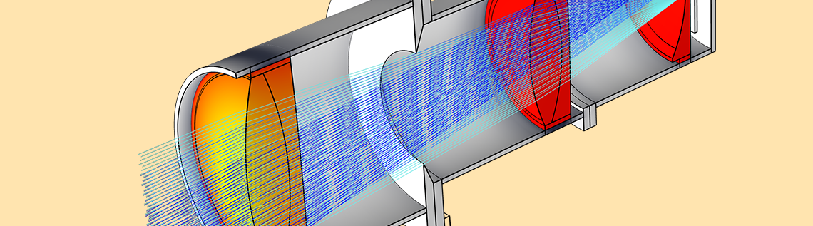
Modern optical systems are often required to operate in harsh environments, including high altitudes, space, underwater, and in laser and nuclear facilities. Such optical systems are subjected to structural loads and extreme temperatures. The most accurate way to fully capture these environmental effects is through numerical simulation via a structural-thermal-optical performance (STOP) analysis. STOP analysis is the quintessential multiphysics problem. In this blog post, we show how to combine structural, thermal, and optical effects using the COMSOL Multiphysics® software.

Describing the Model: A Petzval Lens System Example

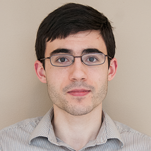
In this example, we consider a Petzval lens system inside of a thermovacuum chamber. The vacuum chamber walls are maintained at a very cold temperature (perhaps to mimic the effects of outer space), while the lens system is looking into an adjacent room at a much higher temperature (possibly emulating a laboratory test). An exploded view of the model geometry is shown below.

The Petzval lens system, barrel, and enclosing thermal shroud. Incident light enters the system through the outermost vacuum chamber window (1) and then through an additional thermal window (2) inside the chamber before reaching the Petzval lens system. The lens system itself consists of two lens groups (3 and 4) and a field-flattening lens (5). The light is focused onto the focal plane (6). The lens system is supported by a barrel (7), which is completely enclosed within the thermal shroud (8).

The ambient surroundings on the other side of the outer vacuum window are a balmy 25°C, while the walls of the thermal shroud are maintained at a brisk -50°C. This fixed temperature might, for example, be maintained by running cold liquid through the shroud, although we will not examine this mechanism in detail and simply treat the walls as a fixed temperature boundary condition. The incoming thermal radiation from the warm ambient surroundings will create a temperature gradient in the lens system and barrel. Intuitively, we might expect the vacuum window to be warmer than the thermal window, which is warmer than lens group 1, and so on, but more quantitative information is needed.

Before we discuss the setup of this model in more detail, let’s consider the different physical phenomena that are at work inside the thermovacuum chamber.

Essential Physics of a STOP Analysis

A STOP model involves a coupling between the following:

• Temperature calculation, using the Heat Transfer in Solids interface or another heat transfer interface
• Structural deformation modeling, using the Solid Mechanics interface or another structural physics interface
• Ray tracing, using the Geometrical Optics interface

The mechanisms that couple these three branches of physics are summarized in the flowchart below.

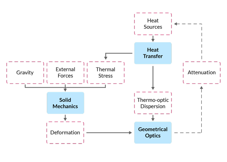
Flowchart of the most significant multiphysics phenomena in a STOP analysis.

Thermal Modeling

The temperature is affected by heat sources and sinks, such as Joule heating or chemical reactions, and by boundary conditions, such as convective or radiative heat exchange with the surroundings.

A special case worth mentioning is the bidirectional (two-way) coupling between ray optics and heat transfer. This arises when a powerful source (from a laser or solar concentrator, for example) undergoes some attenuation in the modeling domain, generating an additional heat source. The example discussed in this blog post is unidirectional: The rays are not powerful enough to generate a significant heat source term through attenuation.

The temperature affects the ray propagation through thermo-optic dispersion, in which the refractive index is a function of temperature. The temperature also indirectly affects the ray paths because thermal stress can cause boundary deformation, as discussed in the next section.

Structural Modeling

Usually, STOP analysis requires a calculation of the structural displacement field. Rays can then interact with the deformed geometry, which might cause them to be reflected or refracted in different directions than in the original, undeformed geometry.

The structural displacement is the result of all forces that are applied to the model geometry, which in this case comprises the lens system and the barrel that holds it in place. The geometry may also deform due to thermal stress, as the temperature changes cause it to expand or contract.

Optical Dispersion Models

The Geometrical Optics interface is used to trace rays as they reflect and refract across boundaries. The refractive index of each material can be a function of both wavelength and temperature. If the lens system is deformed, rays interact with the deformed geometry. In this way, the ray paths are influenced by both thermal and structural phenomena.

The Medium Properties node for the Geometrical Optics interface can be used to select an optical dispersion model, a set of equations and coefficients that define the refractive index as a function of vacuum wavelength (and possibly temperature).

The following screenshot shows the Equation display for the Sellmeier optical dispersion model. The first five rows of equations define the refractive index as a function of the vacuum wavelength. Here, A₁, B₁, A₂, B₂, A₃, and B₃ are the Sellmeier coefficients, which are unique for each type of glass. The last two rows are an additional correction term for the thermo-optic dispersion model. Here, D₀, D₁, D₂, E₀, E₁, and λ_TK are the thermo-optic dispersion coefficients.

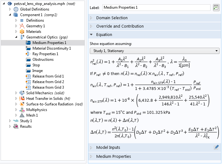
Equations for the Sellmeier optical dispersion model.

One special alternative is worth pointing out here: The Temperature-dependent Sellmeier dispersion model combines the temperature and wavelength dependence into a single equation. This option is most often used as a cryogenic model where the glasses are subjected to an extremely wide range of temperatures.

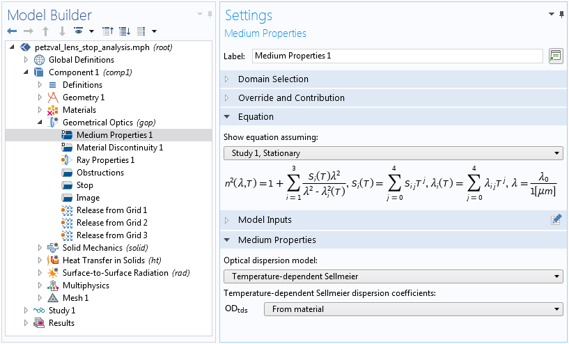
Temperature-dependent Sellmeier coefficients that combine temperature and wavelength dependence into a single expression.

It is usually recommended to select Get dispersion model from material from the Optical dispersion model list. Then, the optical dispersion model will automatically be detected based on which material properties are defined for each material. With this option, you can create a model with multiple glasses from different manufacturers, even if they use different conventions for the optical dispersion model.

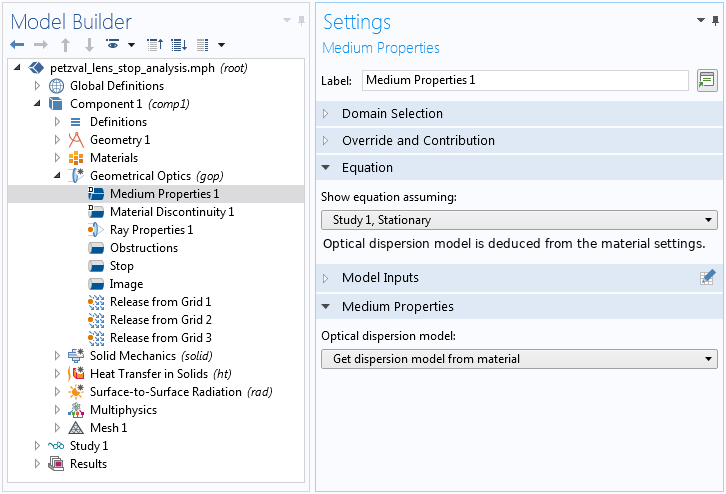
Option to automatically detect the correct optical dispersion model based on which material properties are defined.

Revisiting the Petzval Lens System

Next, let’s consider the example of a STOP analysis for a Petzval lens system inside a thermovacuum chamber, as described earlier.

The heat transfer is modeled using the Heat Transfer in Solids interface for conduction and the Surface-to-Surface Radiation interface for radiative transport between surfaces or between a surface and the ambient surroundings. Only the outside surface of the vacuum window is exposed to the warm ambient surroundings. To couple the conductive and radiative heat transfer to each other, a dedicated Heat Transfer with Surface-to-Surface Radiation multiphysics coupling node is available, as shown below.

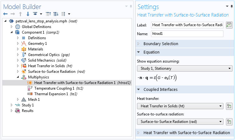
Multiphysics coupling between the Heat Transfer in Solids and Surface-to-Surface Radiation interfaces.

The Surface-to-Surface Radiation interface uses the Diffuse Surface boundary condition on all surfaces, including the lenses; thus, the lens system is assumed to be transparent at optical wavelengths but opaque in the infrared.

The temperature distribution within the lens system and barrel is plotted below. The solid magenta lines indicate the temperature at the center of the vacuum window (1), thermal window (2), lens groups (3-4), and field-flattening lens (5). The blue and red dashed lines are the fixed temperature of the chamber walls (6) and the ambient temperature outside of the chamber (7), respectively.

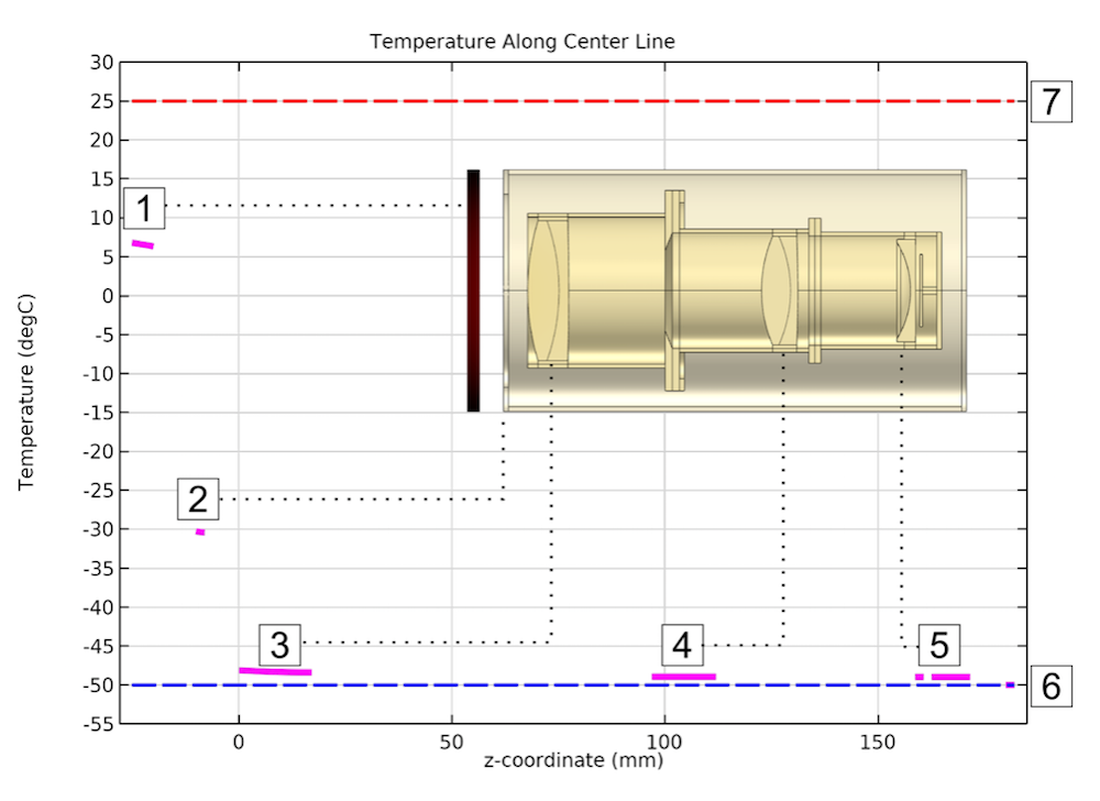
Plot of temperature along the symmetry axis of the lens system, barrel, and chamber.

In this model, the coupling between structural and thermal phenomena is performed by two dedicated multiphysics coupling nodes, as shown below. One of these nodes simply couples the temperature between the two interfaces, and the other specifically adds the thermal stress term to the equations for structural displacement.

Left: Multiphysics coupling to include thermal expansion when solving for the structural displacement field. Right: Multiphysics coupling between the Heat Transfer in Solids and Solid Mechanics interfaces.

To include the thermal expansion when tracing the rays, there is another important step that must be taken. Locate the Ray Tracing study step and make sure that the Include geometric nonlinearity check box is selected. If the check box is not selected, rays will interact with the boundaries of the undeformed geometry, and then the only effect of temperature would be the thermo-optic dispersion model for the refractive index.

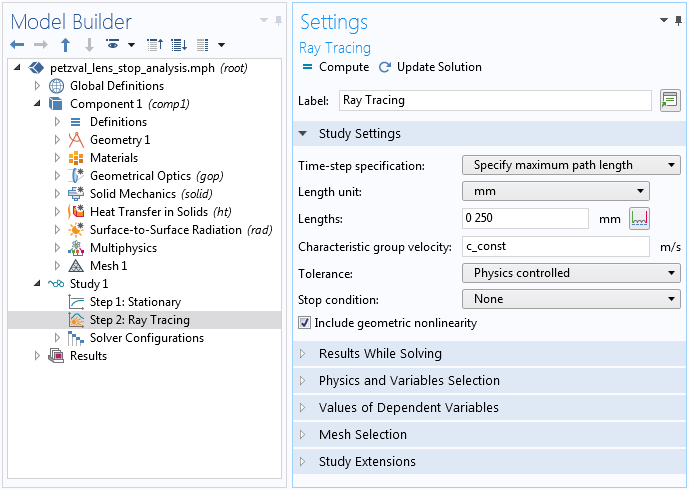
The settings to trace rays in the deformed geometry, accounting for structural deformation.

Ray Diagrams for the Petzval Lens System

Rays are released into the chamber at three different field angles. A ray diagram showing the temperature in a cross section of the lens system and barrel is shown below.

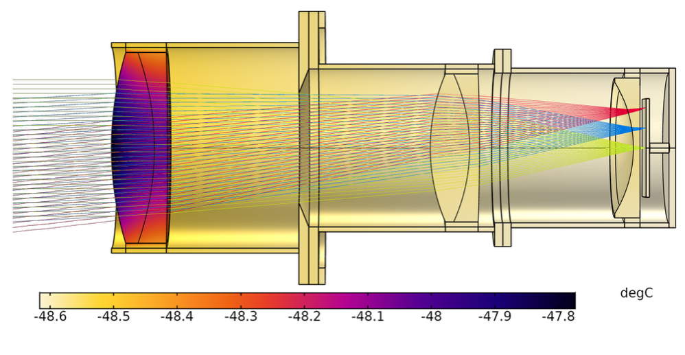
Ray trajectories in the heated Petzval lens system are plotted for three different field angles.

Spot diagrams in the focal plane are shown below. The most symmetric-looking spot diagram corresponds to the zero field angle, while the most asymmetric spot diagram corresponds to the greatest field angle.

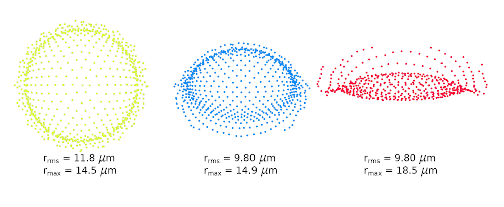
Spot diagrams for three field angles, starting from zero (left).

For comparison, here are the same spot diagrams when the entire apparatus is kept at room temperature (20°C).

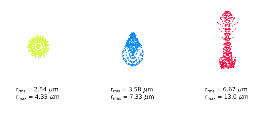
Spot diagrams for three field angles when the lens system is at room temperature.

Concluding Thoughts on Performing a STOP Analysis in the COMSOL® Software

Above, we have demonstrated a STOP analysis of a Petzval lens system enclosed in a cold thermovacuum chamber. A temperature gradient is observed in the lenses because the system is exposed to a much warmer environment outside the vacuum chamber. The cold temperatures significantly increase the root mean square (RMS) spot size.

By the above means of coupling structural, thermal, and optical phenomena in a single model, we’ve suggested an easy-to-use workflow to set up high-fidelity simulations of optical systems under realistic test and operating conditions.

Try it yourself by clicking the button below. This will take you to the Application Galley, where you can download the tutorial documentation and the MPH-file for this example.

To learn more about modeling lenses, read a blog post on how to create complex lens geometries.