The release of version 5.3 of the COMSOL Multiphysics® software includes a new Ray Termination feature to simplify the setup and results analysis for optical simulations with the Ray Optics Module. Use the Ray Termination feature to remove rays that are no longer relevant to the solution, either because they have escaped from the geometry or their intensity is negligibly small. In this blog post, we’ll learn how to use this feature and see how it simplifies ray optics simulation.
Introducing the Ray Termination Feature, New with Version 5.3
The goal of ray termination is to discard rays once they’re no longer useful or relevant to the simulation. By removing rays once they’ve stopped being useful, we can reduce the amount of redundant information in the ray trajectory plots, making it easier to emphasize the more important details in the model.
The simplest way to terminate rays is to stop them as they exit the geometry. The Ray Termination feature stops the rays by creating a fictitious bounding box around the geometry. The bounding box needn’t correspond to any actual geometric entity in the model; it can exist in the void domain outside of all geometric entities and doesn’t require any mesh. In previous versions of COMSOL Multiphysics®, it was instead necessary to create and mesh a number of physical boundaries to block the outgoing rays, or else they would keep propagating until the study was over.
Criteria for Ray Termination
Let’s start with an example of a simple convex lens. Collimated rays are released at a grid of points to the left of the lens. At the lens surfaces, reflected and refracted rays are produced. Suppose we’re only interested in the focused light and not in the reflected light. Then, we can set up a Ray Termination feature with user-defined bounding box dimensions to stop rays that get reflected at the lens surfaces. The settings for this feature are shown below.

Settings window for the Ray Termination feature. User-defined maximum coordinates have been entered for the x– and y-directions.
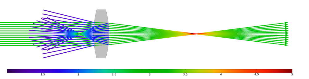
The maximum x-coordinate is much greater in magnitude than the other specified coordinates and significantly greater than the focal length of the lens, so we don’t have to worry about stopping the rays before they reach a focus. One benefit of using the Ray Termination feature is that we don’t have to create or mesh a high-aspect-ratio rectangle to stop the rays; they are simply made to stop at a specified location in space, regardless of whether a physical boundary is defined there. The resulting trajectories are shown below, colored according to the logarithm of the ray intensity.

Rays propagating through the lens and getting stopped by the Ray Termination feature. The color expression is proportional to the ray intensity on a logarithmic scale.
As shown below, letting the reflected rays continue to propagate can obscure or distract from the relevant physics in the model — in this case, the focusing of the refracted light by the lens.
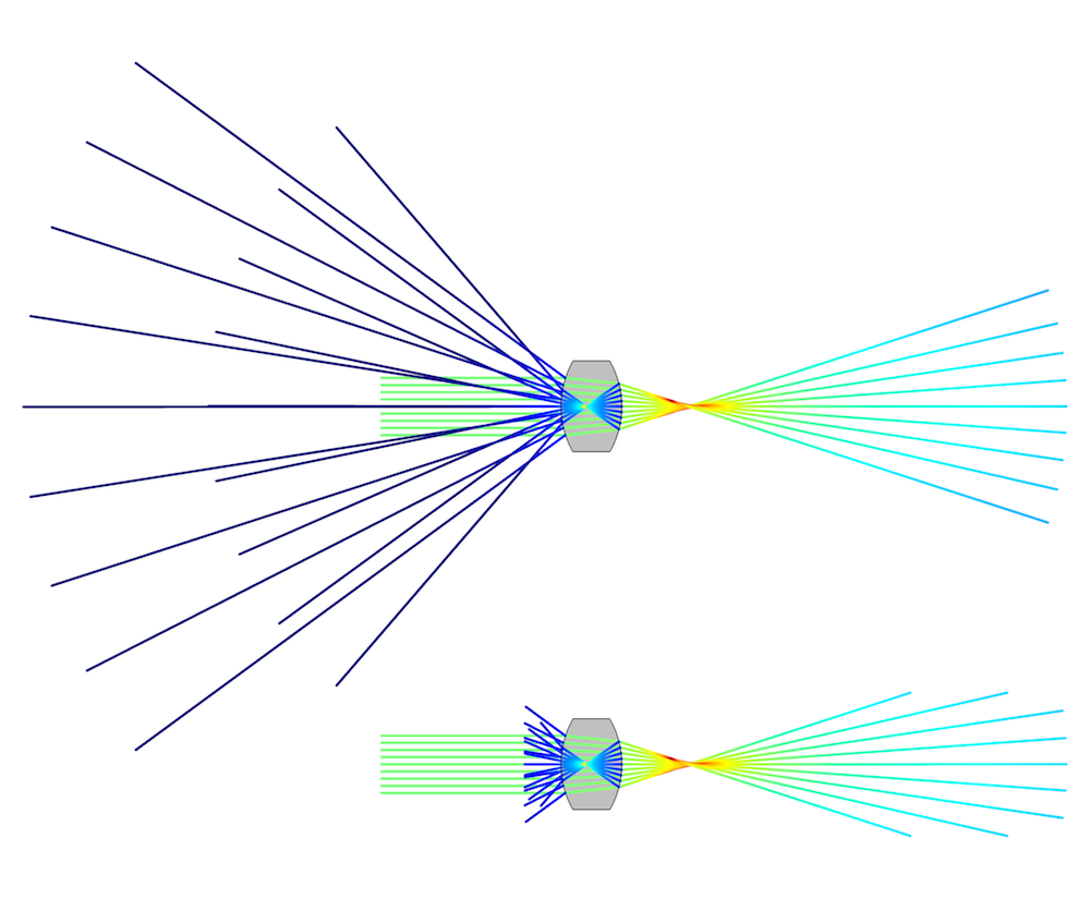
Comparison of the ray trajectories when allowing the rays to continue propagating (top) or using the Ray Termination feature (bottom).
To better visualize how the rays interact with the bounding box, the following screenshot includes edges drawn on three edges of the box. Incidentally, this reveals yet another benefit of using the Ray Termination feature: rays are free to enter the bounding box and only get terminated as they leave. If the three edges drawn in red were modeled as Wall conditions to stop the outgoing rays, we would need to write logical expressions to prevent the wall condition from being applied to the incident rays, which could become rather complicated.

Rays propagating through the lens and getting stopped by the Ray Termination feature. Three sides of the bounding box are drawn in red.
Example: Czerny-Turner Monochromator
The Ray Termination feature is now used in the Czerny-Turner Monochromator tutorial model, available online and in the Application Libraries in the software. I wrote about this example in a previous blog post on ray tracing in monochromators and spectrometers.
The model consists of a grating, two mirrors, and a detector arranged in a crossed Czerny-Turner configuration, as illustrated below. The mirrors, grating, and detector are highlighted in yellow and the path of light is shown in red.
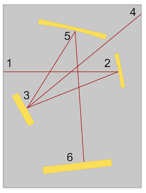
Light paths in the Czerny-Turner Monochromator tutorial.
The numbers denote the different stages of the light path:
- Incoming rays are released from a slit with a conical distribution based on a user-defined numerical aperture.
- The rays are reflected by a collimating mirror. The curvature, position, and orientation of this mirror are such that all reflected rays are parallel to each other.
- The reflected rays hit a diffraction grating, producing rays of several different diffraction orders.
- The reflected rays of diffraction order 0 are all parallel to each other because their angle of reflection is not wavelength dependent. Thus, there is no separation between different wavelengths of light. These rays are aimed away from the mirrors and ignored in results processing.
- However, the rays of diffraction order 1 are reflected in different directions based on free-space wavelength. They are reflected by a focusing mirror.
- Light of different colors is focused to different locations on the detector.
My previous blog post referred to an older version of the COMSOL® software in which it was necessary to create and mesh the air or vacuum domain surrounding the mirrors and grating. Now, however, rays can propagate in the void region outside the geometry, even though that region is not meshed. Therefore, a more minimalist geometry can be used and it is not necessary to indicate the spatial extents of ray propagation with a large rectangular domain, as illustrated below.
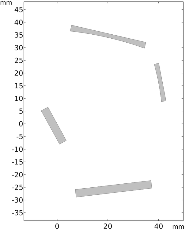
Geometry of the Czerny-Turner monochromator in COMSOL Multiphysics version 5.3.
In this example, the bounding box dimensions for ray termination are automatically determined from the geometry information. For every geometry, the COMSOL® software automatically computes and records the maximum and minimum coordinates in each direction. Together, these coordinates comprise the smallest possible rectangle (in 2D) or rectangular prism (in 3D) with edges parallel to the coordinate axes such that every geometric entity is completely enclosed. This box is illustrated in blue in the following plot.
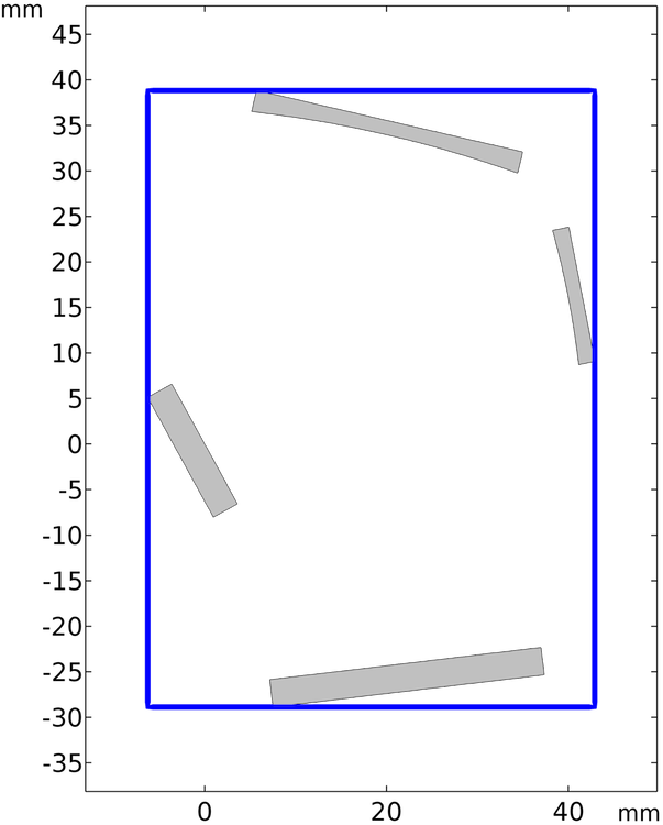
Minimum bounding box to enclose the mirrors, grating, and detector.
With the Ray Termination feature, it is possible to automatically terminate rays as they exit this bounding box defined by the geometry, ensuring that rays are promptly annihilated if there is no chance they will ever touch another geometric entity in the model. This way, we don’t need to modify the bounding box dimensions as we adjust the geometry; the box is automatically resized as needed. To avoid terminating rays when they hit a boundary that coincides with the bounding box, the Ray Termination feature actually extends the box by 5% in every direction. So, rays are terminated as they intersect the red rectangle shown in the following plot, not the blue one.
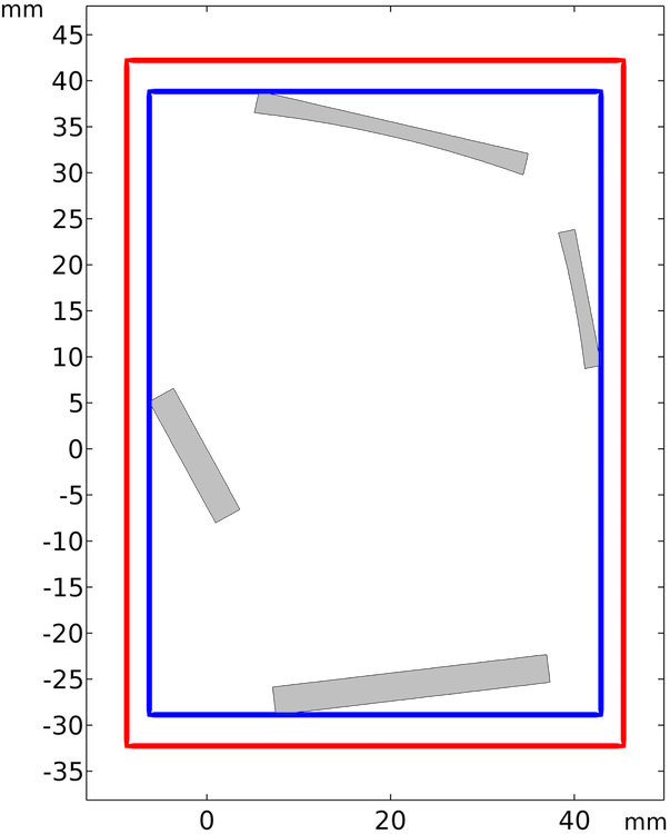
Automatic bounding box used by the Ray Termination feature.
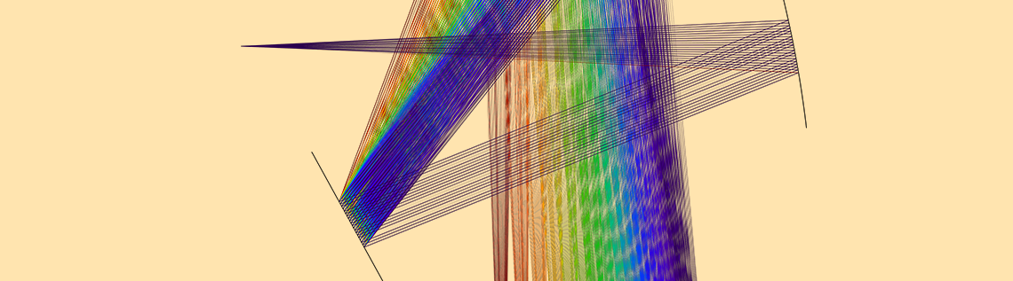
When rays are released into the model, they get reflected by the two mirrors and the grating. The rays of diffraction order 0 get reflected by the grating and then escape the geometry. Note that the rays are terminated as they exit the red rectangle, the bounding box with an extra allowance of 5% on either side.
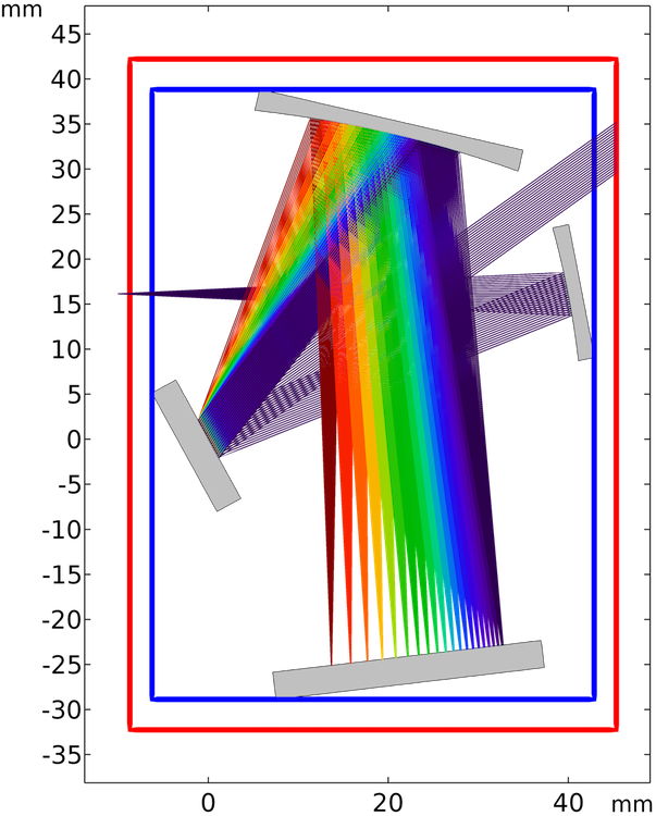
Ray propagation in the Czerny-Turner monochromator. The color expression of the rays roughly corresponds to the actual color of the light.
As in the previous example of a convex lens, the rays actually enter the geometry from a point outside the red rectangle but they aren’t immediately terminated. The bounding box only applies to the rays that are leaving the geometry.
Stray Light Suppression
In the earlier example of rays being focused by a convex lens, we used the Ray Termination feature to eliminate the reflected light at the lens surfaces. This reflected light, sometimes called stray light, is typically minimized through the use of antireflective coatings and might not be of great interest for results analysis. When modeling ray propagation through a single lens, it was easy to terminate the stray light based on the allowed spatial extents of ray propagation because it all propagated to the left, whereas the focused light propagated to the right. For more complicated arrangements of lenses and mirrors, we might want to terminate uninteresting light (like stray light) that is in the same part of the modeling domain as interesting light (like the focused beam), which makes spatial termination more difficult to use.
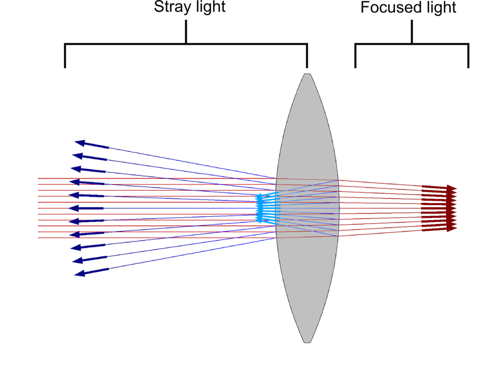
Illustration of stray light and focused light as a collimated beam reaches a convex lens.
Another factor that can be used to eliminate stray light is its intensity, which is usually quite low compared to the refracted light. When the ray intensity is computed, we can specify a threshold intensity; rays get terminated as their intensity falls below this threshold value. This is illustrated in the following plot. Unlike the first example, in which the end points of the terminated rays formed a flat surface along the edge of the bounding box, here the terminated rays form a curved surface, the set of points where the reflected ray intensity becomes sufficiently small to make the ray disappear.
Reflected rays get terminated when their intensity falls below a threshold.
Intensity-Based Termination and Wavefront Curvature
In the previous example, we saw that stray light was annihilated but that the focused light was allowed to continue propagating. This is due to a combination of two effects on ray intensity:
- Convergence or divergence of the propagating electromagnetic waves. Information is stored as the principal radii of curvature of the wavefront associated with each ray.
- Discrete reduction in intensity in accordance with the Fresnel equations when rays are reflected and refracted at boundaries.
The stray light terminated much earlier than the focused light mainly because it had significantly lower intensity to start with. The intensity of the reflected light was about two orders of magnitude smaller than the intensity of the refracted light. However, if given sufficient time, the refracted light would eventually be terminated as well, due to the way intensity falls off as the wavefront diverges beyond the focus of the lens.
This can be seen more clearly in the following animation. Collimated beams pass through two lenses. The top lens has a focal length of 200 mm and the bottom lens has a focal length of 100 mm. Because the focal length of the second lens is shorter, rays begin to diverge sooner. Thus, these rays terminate sooner compared to rays passing through the lens of greater focal length, even though the initial ray intensity is the same for both beams.
Concluding Thoughts on Ray Termination
The new Ray Termination feature extends the usability of the Ray Optics Module because you can use it to easily discard rays that either have negligibly low intensity or simply won’t interact with anything for the remainder of the study. Consider using this feature in your existing ray optics models to simplify geometry setup, avoid wasting computational resources on uninteresting or irrelevant rays, and make the most relevant details stand out clearly during postprocessing.
Further Reading
- See more updates to the Ray Optics Module on the 5.3 Release Highlights page
- Read a blog series on multiscale modeling in high-frequency electromagnetics


Comments (4)
Hannu Välimäki
August 16, 2017Hi!
Is there a convenient way to create aperture stops in comsol ray tracing? Like making a geometric hole in the optical path and defining the material around the hole as fully (or very strongly) absorbing? Playing around for some time, I have not find a way, yet.
Christopher Boucher
August 17, 2017 COMSOL EmployeeHi Hannu,
Rather than defining the aperture stop as a strongly absorbing domain, it is usually more convenient to define aperture stops as surfaces where you apply the “Wall” boundary condition. This condition can terminate rays that hit the selected boundaries.
Best Regards,
Chris
hazem hattab
February 1, 2018Im building a model of vacuum tube solar thermal with reflector i need to use several solar angle of incidence how to define solar ray in a several angle in one study
Ernesto Katongo
April 8, 2026What is the correct, physically consistent way to compute reflectance in the Geometrical Optics interface?
Specifically:
Should reflection be measured using accumulators at a boundary?
Or by identifying rays that leave the domain (escaped rays)?
How can we ensure the result corresponds to hemispherical reflectance (as in PV Lighthouse)