Two Methods for Modeling Free Surfaces in COMSOL Multiphysics®

There are four methods for modeling free liquid surfaces in the COMSOL Multiphysics® software: level set, phase field, moving mesh, and stationary free surface. In the first part of this blog series, we discuss the level set and phase field methods, which are field-based methods that describe almost any type of free liquid surface. In part two, we will compare the results from this post with those obtained using the Moving Mesh interface for solving free surface problems.

What Are the Level Set and Phase Field Methods?

The level set and phase field methods are both field-based methods in which a free fluid surface is represented as an isosurface of the level set or phase field functions. The free liquid surface corresponds to the phase boundary between the liquid and the gas and is represented on a fixed mesh.

The figure below shows the surface of two droplets in a channel, taken from the droplet breakup model in the Application Library of the add-on Microfluidics Module. We can see in this plot that although the surface of the droplet is very sharp, the elements around the droplet do not adhere to the droplet’s surface.

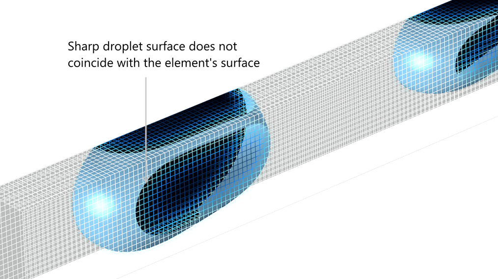
The droplet surface does not coincide with the surface of the elements, neither in the level set method nor in the phase field method.

The level set and phase field functions are both advected by the velocity vector computed by the Navier-Stokes equations. For both the level set and the phase field methods, this looks like:

(1)

Note that we are using Φ for both the level set and phase field functions. The right-hand side of the equation, F, is where the two methods differ. In the original level set method, F = 0, which gives a pure advective transport equation. However, the numerical solution with F = 0 is unstable and of small practical use in most cases. Instead, terms with higher-order derivatives of Φ, designed to keep the interface compact, are introduced in F in the level set method.

In the phase field method, F represents a term that tries to minimize the free energy of the system. Also, higher-order derivatives of Φ are introduced in this term. In fact, the source term in the phase field equation includes fourth-order terms. This means that, for practical reasons, the equation is often broken up into two equations, where an auxiliary dependent variable is defined as a function of the second derivatives of Φ. This is also what is done in COMSOL Multiphysics.

Both methods introduce the source term into the Navier-Stokes equations that originate from the surface tension at the free liquid surface. In the level set method, the curvature of the level set isosurface that represents the free boundary is used to describe surface tension. In the phase field method, the contribution to the Navier-Stokes equations from the surface tension is calculated from the chemical potential, which yields the surface tension and the gradient of the phase field function close to the interface.

The properties of the fluid transition smoothly from liquid to gas over a given value of the level set or phase field functions; i.e., the value that represents the free surface.

The level set function, Φ, varies between 0 and 1 across the free surface and is constant at 0 or 1 in the bulk of the two fluids. The level set function can, for example, be 0 for the liquid and 1 for the gas phase. The free liquid interface; i.e., the phase boundary between liquid and gas; corresponds to the value of the level set function Φ = 0.5. The density is thus a function of the level set function according to:

(2)

As well as the dynamic viscosity:

(3)

We can see in the two equations above that when Φ = 0, we get the properties of fluid 1 (for example, the liquid) and when Φ = 1, we obtain the properties of fluid 2 (for example, the gas). We obtain a smooth transition of fluid properties across the free surface; i.e., as smooth as the level set function.

The phase field function, Φ, varies between -1 and 1, where the free liquid surface is the isosurface for Φ = 0. The computation of the viscosity and density is done in an analogous way to the level set method, but with a different expression, since the phase field function varies between -1 and 1.

Settings in the Level Set and Phase Field Interfaces

The Level Set and Phase Field interfaces contain a number of parameters that need tuning in order for the methods to perform optimally. The values of these parameters depend on the modeled system and the numerical discretization of the equations. The size of the geometry (length, width, and depth); properties of the fluids; wetting of the walls; initial conditions; operating conditions; and size of the elements in the created mesh all have an impact on the selection of the model settings.

The Level Set Interface

Let’s start with the level set method’s settings. The reinitialization parameter, γ in the user interface, makes sure that the gradients in the level set function are concentrated to the free surface over time; i.e., to the interface between water and air in our example below. It does not set the thickness of the surface, but it makes sure that the variations of the level set function are contained within this thickness. If we set this value too low, variations in the level set function can be entrapped in the bulk of one of the fluids, creating liquid-gas interfaces out of nowhere. A value that is too high tends to give small time steps and large computation times.

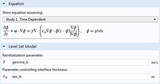
The Settings window for the Level Set interface.

The interface thickness parameter, denoted ε in the user interface, is more intuitive to understand. It simply controls the thickness of the region where the variations of the level set function are obtained. A large thickness smears out the shape of the free surface. The problem becomes easier to solve, but accuracy in the shape of the free surface is lost. A small value of ε yields a compact representation of the surface but requires a corresponding resolution of the mesh. There is no point in setting a value that is much smaller than the mesh element size, since the interface then becomes ragged and unresolved surface tension forces might cause spurious velocities. The value of ε should be set approximately to the same value of the largest elements close to the surface.

The Phase Field Interface

If we now look at the phase field method, the interface thickness parameter, ε, is almost identical to the level set method above and the same reasoning can be applied to the selection of its value.

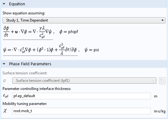
The settings for the Phase Field interface.

The mobility tuning parameter for the phase field method, χ in the user interface, determines in a certain way the diffusivity of the phase field. This value has to be large enough for the phase field equation to be stable but small enough to give a sharp interface. The proper value is proportional to the speed at the surface and inversely proportional to the coefficient of surface tension.

(4)

This means that once we have found a proper value of χ for a certain set of operating conditions, we can use the relation above to set χ for a new set of conditions.

Modeling a Free Liquid Surface

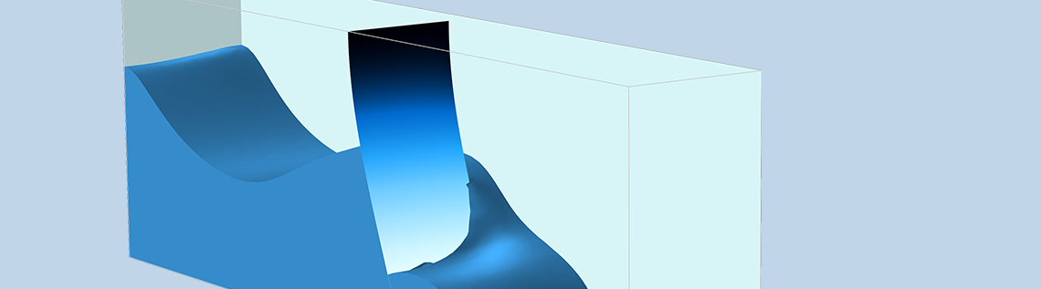
The figures below show the example problem that we are going to use to investigate the level set and phase field methods for modeling free surfaces in COMSOL Multiphysics.

A solid bar is half immersed in water in a small channel. The bar is put into motion back and forth, tangential to the water surface, in order to generate a gentle wave on the water surface. The dimensions of the channel and bar are small enough to keep the flow laminar.

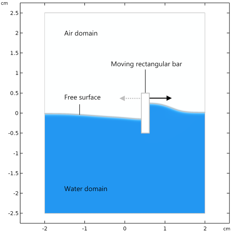
Geometry and definition of the example problem.

Note that the moving mesh functionality is used to prescribe the movement of the little rectangular bar back and forth on the surface. However, in the level set and phase field methods, the mesh is not moved with the liquid surface.

Here are a few remarks about the model implementation in COMSOL Multiphysics:

• We add gravity as a source in the momentum equations
• We add a reference and a point constraint for the pressure field
• In order to compare results, we select Navier slip conditions for the walls and use a slip length equal to the size of the element length

Simulation Results for the Level Set and Phase Field Methods

The results for the flow field and the shape of the water surface are shown below for the following times: 0.07 s, 0.57 s, and 1.0 s. The flow streamlines and the shape of the water surface are in decent agreement for both methods at the respective times. There is a slight difference in the maximum velocity and in the height of the water surface, which may be explained by the fact that the two methods treat surface tension differently.

There are also some differences in the streamlines after longer times, for example, in the recirculation zones at t = 1.0 s. The phase field method tends to give a slightly calmer behavior of the surface. The level set method computes the surface tension force from the curvature of the surface, which is obtained from the gradient of the level set function. This gives a more “spiky” surface force compared to the smoother force obtained with the phase field method.

Results from the level set (left) and phase field (right) methods after 0.07 s (top), 0.57 s (center), and 1.0 s (bottom).

We can also visualize the full results from the simulation in an animation for the period from 0 s to 2 s. We can see that although the movement of the rectangular bar causes vigorous stirring, the free surface never breaks.

An animation created from the solution of the problem using the phase field method.

The level set and phase field methods also compute the flow field in the air domain above the free liquid surface. We can see that the movement of the rectangular bar leads to a vigorous flow field pattern that is continuous over the phase interface.

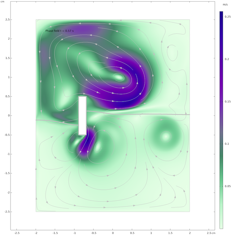
The flow field in the water and air domains as computed with the phase field method after 0.57 s.

If the agitation of the surface is increased so that it becomes more vigorous, then the surface can break up and later coalesce, which is shown in the animation below. This is also one of the benefits with the level set and phase field methods: It is relatively easy to deal with topology changes in the free surface in any of these two methods.

The agitation with the rectangle-shaped bar is increased both in frequency and amplitude until a small wave breaks and generates entrapped air pockets in the water phase.

Although the level set and phase field methods are similar, the treatment of the surface tension has a large impact on the stability of the two methods, at least in the implementation in COMSOL Multiphysics. For problems involving a strong effect from surface tension, the phase field method shows better performance regarding computation time compared to the level set method. The reason for this difference is that the computation of the surface curvature in the level set method forces the time-dependent solver to take substantially smaller time steps compared to the phase field method.

In our example, the time steps are on average five times larger in the phase field method, which results in a five-times-larger computation time for the level set method. So, for free surface problems at a small scale and for laminar flows where surface tension has a large impact (for example, in microfluidics), the phase field method is in general a better option.

Adaptive Mesh Refinement and Free Surfaces

In the 2D example that we have investigated in this blog post, the mesh is dense enough over the whole region where the free surface is expected to be found for the level set and phase field method. However, for 3D cases, we cannot always afford this type of resolution. One approach is to use the functionality for adaptive mesh refinement, which automatically creates a denser mesh according to whatever function we choose.

For example, the animations below show the mesh adaption according to the location of the largest gradients in the velocity (left) and according to the largest gradient in the phase field function (right). The plot shows both the air and the water phases. Note that the adaptive meshing with respect to the shear rate gives a refined mesh in the air phase and not that much in the water phase. In this case, we are interested in the water phase so we have to change the error indicator for adaptive meshing by scaling with the phase field function.

Adaptive mesh refinement with velocity gradients as error indicator (left) and with the phase field gradient as error indicator (right).

Moving Mesh and Free Surfaces

This blog post discusses the two field-based methods for modeling free surfaces: the phase field and the level set methods. In the second blog post in this two-part series, we will compare the modeling of free surfaces using moving mesh with the field-based methods shown here. Stay tuned!

Update: Part two is now live and you can read it here.

Next Steps

Learn more about the specialized features for simulating fluid flow available in the CFD Module, an add-on to COMSOL Multiphysics, by clicking the button below.

Further Reading

• Try it yourself: Download the MPH-file from the Application Gallery
• Read about other practical applications of the level set and phase field methods on the blog:
  • Modeling a Sphere Falling on a Water Surface
  • Designing Inkjet Printheads for Precise Material Deposition

Editor’s note: This blog post was updated on 5/25/2018 to include a link to the MPH-file of the example model, which has been added to the Application Gallery.