
As we saw previously in the blog entry on Solving Nonlinear Static Finite Element Problems, not all nonlinear problems will be solvable via the damped Newton-Raphson method. In particular, choosing an improper initial condition or setting up a problem without a solution will simply cause the nonlinear solver to continue iterating without converging. Here we introduce a more robust approach to solving nonlinear problems.
Editor’s note: The information in this blog post is superseded by this Knowledge Base entry: “Improving Convergence of Nonlinear Stationary Models”
Example of a Nonlinear Problem
Consider again the system of a force applied to a spring with nonlinear stiffness:
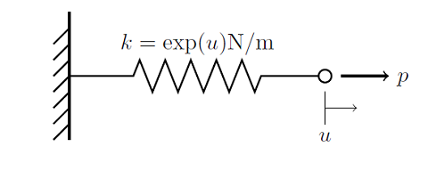
We can solve this problem with the damped Newton-Raphson method as long as we choose an appropriate initial condition (earlier we chose u_0=0). In the other blog entry, we noticed that choosing an initial condition outside of the radius on convergence, any point u_0\le-1 for example, will cause the solver to fail. Now, for this single degree of freedom problem we can easily determine the radius of convergence, but for typical finite element problems it would be much harder. So instead of trying to find the radius of convergence, let’s instead apply a little bit of physical intuition to this problem.
Load Ramping Improves Robustness
Here we are applying a load, p_f, to a system and we are trying to find a solution by starting from an initial condition, u_0. But what happens if we apply a load p=0? Newton’s First Law tells us that a system under no load will have no deformations. So what happens if we apply a load, p_1, of magnitude infinitesimally larger than zero? It would be reasonable to assume that the Newton-Raphson method, starting from u_0=0, will be able to find a solution, u_1. It is also reasonable to say that we can then increment the load to p_2 such that p_1<p_2<p_f and again find a solution u_2, as long as the load increment is small enough. Repeating this algorithm, we will eventually get to the final load p_f, and our desired solution. That is, starting from a zero load, and zero solution, we gradually ramp up the load until we achieve the desired total load. This procedure is plotted in the figure below. The dark arrows indicate where the Newton-Raphson iterations start for a particular load value.
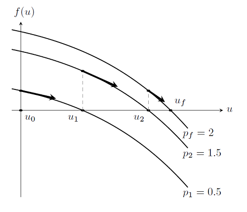
This algorithm is also referred to as a continuation method on the load. This gradual ramping up the load from a value close to zero is often a more robust approach to solving nonlinear problems via the damped Newton method, since the previous solutions are good initial guesses for the next step.
With this algorithm, we not only have a good way of addressing the issue of finding a good starting point for the Newton-Raphson iterations, we also have an algorithm that is useful for the case of a problem that does not have a solution. Consider again the problem where the spring gets weaker as it is pulled, where f(u)=2-\exp(-u)u as discussed previously. This problem does not have a solution. In this case, we can analytically determine that for any load p>\exp(-1) there is no solution. But if we use a smaller load, then the system is stable. In fact, in our scenario the system is bi-stable; there are two solutions for every load p \le \exp(-1). Although, we are probably only interested in the branch we get to starting from p=0 and u_0=0. Let us plot out f(u):
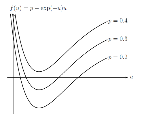
Now let’s also assume that we do not know that the peak possible load is at p = \exp(-1), and examine what happens when COMSOL tries to solve this problem for p = 0.2, 0.3, 0.4. If we plot out f(u) for p = 0.2, 0.3 we see that for p = 0.4 there is no solution to be found. The continuation solver in COMSOL will then automatically perform a search over the interval between the last successful load value and the next desired load step. That is, the solver tries to backtrack to find an intermediate solution that can then be used as a starting value for the next step. This algorithm is always used whenever the Continuation Method feature (or the Parametric Sweep feature) is used on a single parameter when solving a stationary problem. In that case, the solver will be able to find the approximate failure load of the system, which is also very useful information.
Summary and Concluding Thoughts
We have now introduced the concept of load ramping and using the continuation method to improve the robustness of the Newton method. Since a system with no load has a known solution, we have seen that this technique can eliminate the question of what value to choose for the initial condition. We also learned that it is possible to approximately find the failure load. For these reasons, load ramping is one important technique that you should understand when setting up and solving nonlinear static finite element problems.
COMSOL Log File
Let’s take a look at a log file from a nonlinear finite element problem. We’ll set up and solve the problem described above, of a nonlinear spring that gets weaker as we pull on it. We know that this problem does not have a solution, so lets see what happens:
Stationary Solver 1 in Solver 1 started at 15-Jul-2013 11:26:46.
Parametric solver
Nonlinear solver
Number of degrees of freedom solved for: 1.

Parameter P = 0.2.
Symmetric matrices found.
Scales for dependent variables:
State variable u (mod1.ODE1): 1
Iter      ErrEst     Damping    Stepsize #Res #Jac #Sol
   1        0.18   1.0000000           1    2    1    2
   2       0.013   1.0000000        0.22    3    2    4
   3    6.5e-005   1.0000000       0.015    4    3    6
Parameter P = 0.3.
Iter      ErrEst     Damping    Stepsize #Res #Jac #Sol
   1       0.025   1.0000000        0.21    7    4    9
   2     0.00069   1.0000000       0.031    8    5   11

Parameter P = 0.4.
Iter      ErrEst     Damping    Stepsize #Res #Jac #Sol
   1        0.89   1.0000000         2.7   11    6   14
   2         0.3   0.8614583        0.76   12    7   16
   3         0.2   0.8154018        0.43   13    8   18
   4        0.31   0.4194888        0.42   14    9   20
   5        0.86   0.0836516         0.9   15   10   22
Parameter P = 0.325.
Iter      ErrEst     Damping    Stepsize #Res #Jac #Sol
   1       0.089   1.0000000         0.4   18   12   26
   2       0.014   1.0000000        0.13   19   13   28
   3      0.0003   1.0000000       0.018   20   14   30

Parameter P = 0.375.
Iter      ErrEst     Damping    Stepsize #Res #Jac #Sol
   1       0.099   1.0000000        0.32   23   15   33
   2       0.079   0.9390806        0.19   24   16   35
   3         0.2   0.3028345        0.24   25   17   37
   4        0.94   0.0302834        0.95   26   18   39

... SOME PARTS OF THIS LOG FILE OMITTED ...

Parameter P = 0.368359.
Iter      ErrEst     Damping    Stepsize #Res #Jac #Sol
   1       0.046   1.0000000       0.057   80   49  112
   2       0.061   0.3013806       0.072   81   50  114
Stationary Solver 1 in Solver 1: Solution time: 0 s
                                 Physical memory: 471 MB
                                 Virtual memory: 569 MB
The solver also reports an error:
Failed to find a solution for all parameters,
even when using the minimum parameter step.
No convergence, even when using the minimum damping factor.
Returned solution is not converged.
The beginning of the log file is as before, except that the solver now reports that the Parametric Solver is being called. We see that, for P = 0.2 and P = 0.3, the solver completes. For P = 0.4, the solver fails and then automatically backtracks to try to find intermediate points that solve. Some of the intermediate steps are omitted for brevity, but we see that the parametric solver ends up very close to the analytic solution for the peak load. From this information, we could re-solve the problem with a different set of parameters and get a better idea of how the system behaves as we approach the failure load, which is often useful information.


Comments (2)
Jiang Fan
December 9, 2013Thanks Walter, it gives us deeper understanding of COMSOL.
Deokhan Kim
March 24, 2017Thanks a lot. Your postings are very helpful.