Guest blogger Bojan Jokanović of SGL Carbon GmbH discusses the utilization of simulation for the analysis of material structures based on optical microscopy images.
It is well known that the properties of materials are strongly dependent on their structure. A material microstructure typically contains two or more phases with substantially different properties. Each production step may leave its marks in the material structure in the form of the shape and volume fraction of pores, orientation and size of inclusions, etc. That’s why quantitative structure characterization is important for the evaluation of the material properties and its performance in the intended applications.
Synthetic Graphite: A Useful and Complex Material
SGL Carbon, as a world-leading company in the development and production of carbon-based solutions, delivers products and solutions to many industries, including solar, semiconductor, car manufacturing, ceramics, and metallurgy. Many of our solutions are based on synthetic specialty graphites. Synthetic graphites have high thermal and electric conductivity, high temperature stability in inert atmospheres, and superior chemical resistivity — thus they are extensively used in applications involving high temperatures and aggressive chemical environments.
The subclass of isostatic-pressed, fine-grain graphite (Fig. 1) has the finest structure and the most isotropic form of all artificial graphites. It is commonly used for applications where the mechanical properties of other graphites are inadequate.
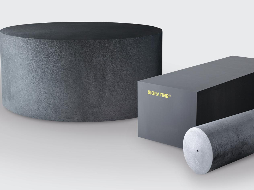
Figure 1. Isostatic-pressed graphite of type Sigrafine® (registered trademark of SGL Carbon SE).
The fine structure of this type of graphite complicates the quantitative optical analysis, and only through the application of modern digital image technology (including simulation) is it possible to distinguish between the different material qualities.
Analyzing Isostatic-Pressed Graphite Materials with Simulation
In our work, we used optical microscopy images (Fig. 2), because it is possible to obtain a large amount of these data in a short period. In the past (e.g., B. Jokanović, keynote talk at the COMSOL Conference 2019 Cambridge), we showed that more detailed analysis is possible using 3D images coming from CT scans. However, the analysis of 3D images requires a huge amount of resources, particularly extensive random access memory and also a large effort for scanning, modeling, and simulation, which limits the amount of samples that can be analyzed.
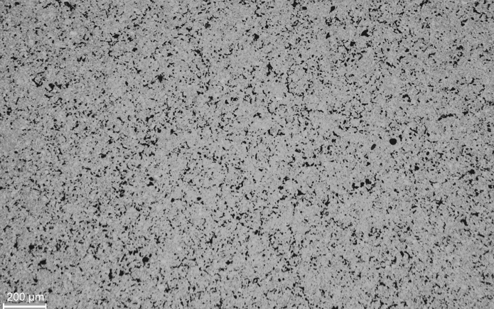
Figure 2. Optical microscopy image of the isostatic-pressed graphite.
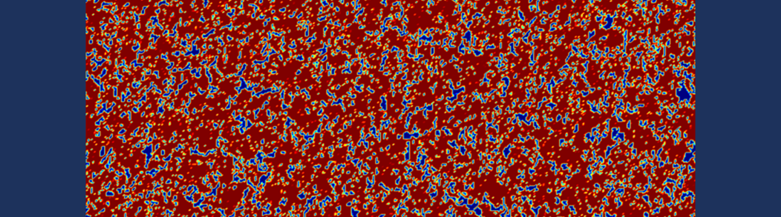
The 2D images are segmented into a void and a solid phase based on the difference in the histogram values of these two phases. Consequently, the images are imported into the COMSOL Multiphysics® software (Fig. 3), and a step function with narrow transition is used to separate the material into two distinctive phases. The mesh size is tuned to the pixel size to encompass the phases correctly.
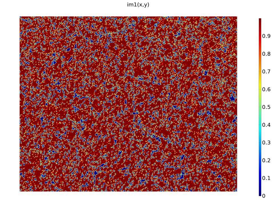
Figure 3. Image imported in COMSOL Multiphysics, containing continuous phases between the solid (red) and voids (blue). Using a sharp step function, the transition phase could be eliminated.
Using a diffusion equation, the homogenized material properties can be determined. Since the void phase in 2D images is discontinuous, to determine the transport properties through the void phase, a small positive conductivity value has to be assumed for the solid phase; in this case, a factor of one million smaller than that of the pores.
Editor’s note: We describe in detail how to manipulate a binary image to compute the effective permeability and porosity in the Pore-Scale Flow model.
Figure 4 shows two materials with equal porosity and yet a 35% difference in the gas diffusivity through the pores. Clearly, in applications with considerable gas corrosion, which are quite common for graphite, this may be a limiting factor for the material stability.
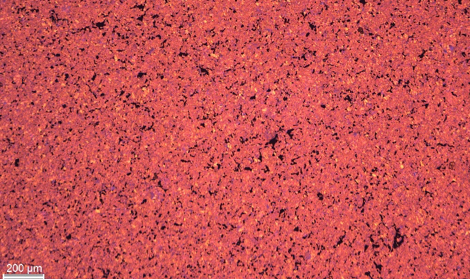
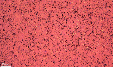
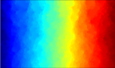
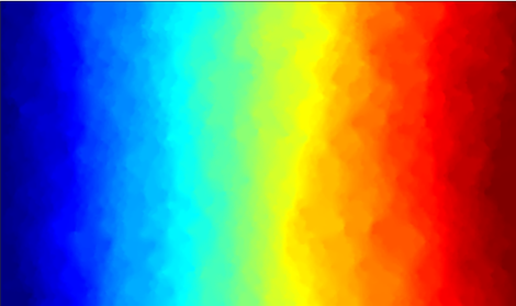
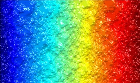
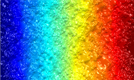
Figure 4. The right sample has approximately the same density as the left sample, and yet 35% lower gas diffusivity. The colors stand for the gas concentration (zero to one).
Through the application of LiveLink™ for MATLAB®, the process is automated so that thousands of images can easily be imported and analyzed.
It is important that the physics is also interchangeable, so that the model can easily switch to the calculation of the elastic behavior, thermal and electrical conductivity, etc. It is thus possible to determine all relevant properties for the intended application and rate the samples coming from the same family based on the simulation results.
Calculating transport in one direction only, the anisotropy of the sample can be evaluated (Fig. 5). In our case, the anisotropy of the void phase is much higher than the anisotropy of the solid phase (Fig. 6), so that the orientation of the graphite pieces can be important for the lifetime of the material in some applications. Also, the small variations of density that are typical for these materials may considerably influence the permeability and diffusivity of the material.
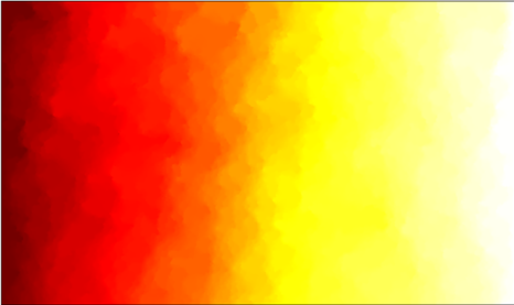
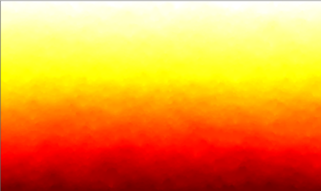
Figure 5. Potential field for the transport through voids in the horizontal (a) and vertical (b) directions.
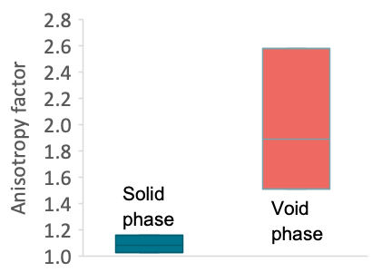
Figure 6. Anisotropy factor of the solid and the void phase.
The differences between the samples coming from the nearby positions are rather small compared to differences between the samples having different processing histories, so the images can be considered representative for a certain material.
Together with our modernly equipped lab, we established a full process that we use for our internal material analysis and also commercially offer to our customers (Fig. 7).
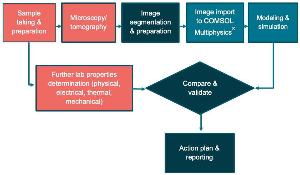
Figure 7. Flowchart of the material analyses that are internally used and commercially offered.
About the Author
Bojan Jokanović works as a senior expert, modeling in the SGL Carbon company in Meitingen, Germany. He finished his PhD at the Technical University Clausthal in Germany, working on the modeling of the oxidation of carbon fiber ceramics. His field of research comprises process modeling and optimization, development of new measuring techniques and tools, as well as the digital characterization of materials. Beside this, he has a rich experience in the field of operations research.

Comments (6)
Said Bouta
March 10, 2020Hi Bojan,
It is good that the Comsol allows to simulate a real image, if we have a sequence of images of a material for example which was obtained by the Micro-tomograph, is it possible to import into Comsol and if possible simulated ?
Bojan Jokanovic
March 11, 2020Hi Said,
It is possible to import 3D images into COMSOL. Depending on complexity of the material, it may be difficult to calculate the complex physics into it. For simpler, it works fine, as long as enough RAM is available. For instance steady state well-posed problem with 10 million DOFs can be calculated in one or few minutes. It is however certainly more difficult to prepare the model, so that the full automation is much more challanging. If you have some certain problem, you can contact us directly.
Joel Shor
March 27, 2020Hi Bojan, do i understand that you can take a micrograph of a isopressed sample cross section and with comsol calculate accurately properties such as thermal conductivity and tensile strength? How well do predictions and data compare? Thank-you,
Joel
Emmanuel CINI
April 1, 2020Hi Bojan,
Further to the question of Joel Shor, I guess that the “small positive conductivity […] assumed for the solid phase” might have an impact on the comparison between calculated and experimental properties.
Did you perform any sensitivity analysis (impact of image processing parameters eg. mesh-pixel sizes tuning, virtual conductivity of solid phase…) regarding the quality/agreement of numerical simulations with physically measured data ?
Regards.
Emmanuel.
Bojan Jokanovic
April 1, 2020Hi Emmanuel & Joel,
Thanks for your interest in my research. You asked similar question, so I’ll try to answer both your questions with one post…
Last year we tested the properties coming from CT scans with our lab measurements and had a good agreement, especially for larger volumes, with fine structure. In this study we were focused on relative differences between the samples coming from very similar production conditions. There is a difference between the results in 2D and 3D, yet the trend is the same, which simplifies the analysis, since there is no need to test thousends of 3D scans, which would take quite a long time. Regarding sensitivity, we wanted to have well separated phases, which would be artificially homogenized using coarser mesh. Depending on the sensitivity of the property this can have large effect. Regarding virtual conductivity of the solid phase… assume you set zero… obviously since the pores are not interconnected in 2D images (contrary to 3D) you would have no flow, meaning the total conductivity is zero. It is thus necessary to set small positive value (for all samples the same) to get physically correct results. Tensile strength is not calculated but only stiffness, since the tensile strength depends more on the size of the sample and we deal yet with small samples. I hope this answers your questions.
Regards,
Bojan
Yanbin He
May 17, 2021Hi Bojan,
Can you share a demo model?
All the best