In a previous blog post, we introduced the principle behind the operation of rapid detection tests based on lateral flow assay (LFA). In this post, we will look at what such a test could look like for COVID-19 detection. In addition, we present three models that can be used for understanding these simple, robust, yet quite advanced microlaboratories.
How Do COVID-19 Tests Work?
When the body is infected with the coronavirus, SARS-CoV-2, the immune system quickly reacts by forming antibodies. Dendritic cells may present virus antigens to allow recognition by T-cells. T-cells may activate B-cells to secrete antibodies that target the antigen (Ref. 1). Among the first to form are the so-called IgM antibodies. These antibodies attach to the surface of so-called antigens on the virus particles as soon as they come close. In the case of the coronavirus, the antigens can be the spike proteins at the surface of the virus (S antigen). Once attached to the antigens, the antibodies block the spike proteins of the virus, impeding them to attach and infect human cells. This neutralizes the virus, since it is not able to replicate outside of an infected cell. There are a number of different antibodies that may target different antigens. Note that there are also other mechanisms for fighting the infection. In addition, T-cells that recognize the virus may also target infected cells directly. They can instruct the cells to self-destruct or they may kill the infected cells, thus also neutralizing the virus.
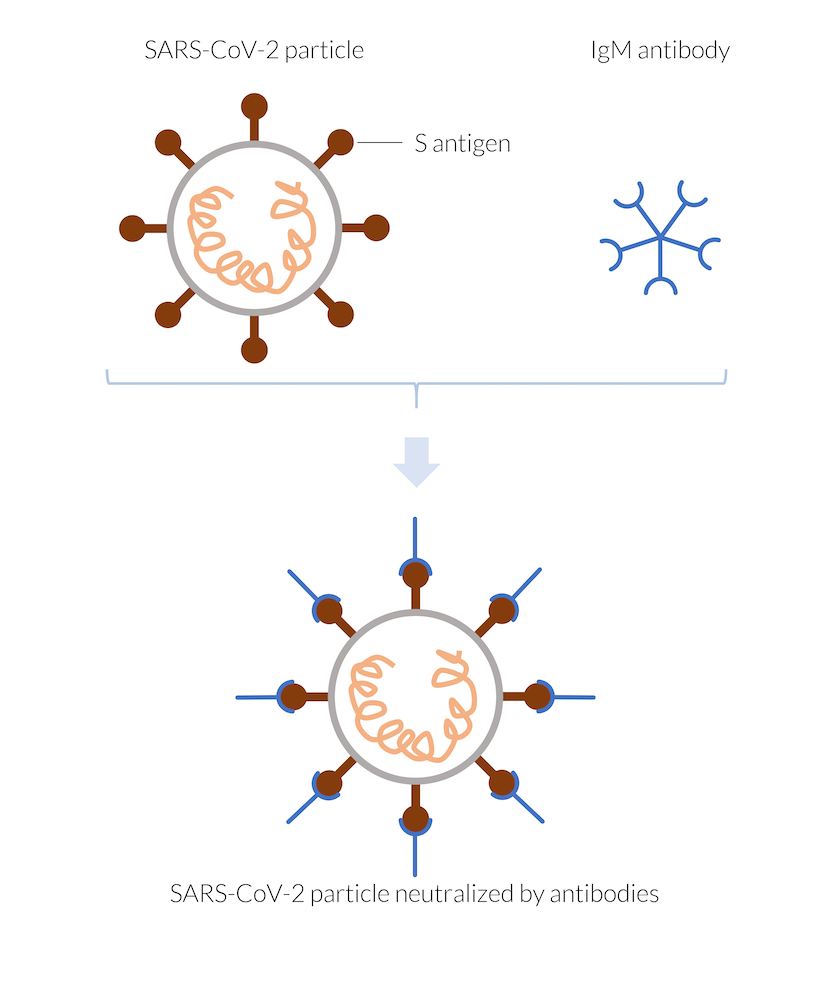
The IgM antibodies manufactured by the immune system attach, for example, to the spike antigen (S antigen) of the SARS-CoV-2 virus particle, thus neutralizing the particle. The neutralized virus cannot enter a human cell and therefore cannot replicate. The virus particle is destroyed.
The IgM antibodies patrol the body in groups of five, forming small particles (or large molecules), attaching to every virus particle they encounter. Later in the infection, the immune system also forms other antibodies, for example, IgG, that patrol the body on their own and fasten to every virus particle they see. The IgG antibodies take longer to manufacture by the body, but they also last longer and grant immunity as long as they are present.
Some of the LFA rapid detection tests for COVID-19 are based on the detection of both IgM and IgG antibodies. These are the tests that are investigated in the model featured in this blog post.

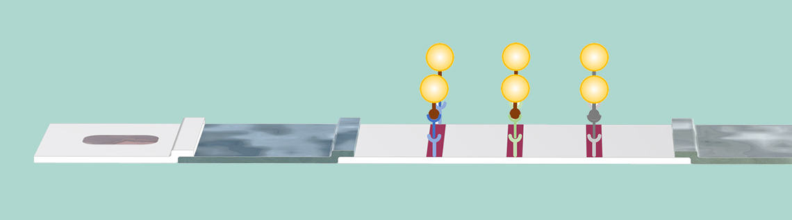
The sample contains the human antibodies IgM and IgG, created due to COVID-19 infection. An animal antibody is also added to the sample liquid with the buffer solution. The test lines have immobilized antibody detectors on the three different areas. Note that the test lines are not yet visible.
The patient’s blood (or saliva) may be applied to the sample well followed by an application of the buffer, by dripping a couple of droplets of buffer in the sample well.
The sample is transported by the capillary forces to the conjugate pad. Here, the IgM and IgG antibodies attach to a conjugate label. A conjugate label may be a gold nanoparticle that has SARS-CoV-2 antigens on its surface. Two different complexes are then formed:
- IgM with the conjugate (IgM-C)
- IgG with the conjugate (IgG-C)
These complexes are dissolved in the sample liquid.

The IgM and IgG antibodies pick up the gold particles by attaching to the SARS-CoV-2 antigen on the particle surface. Also, the animal virus antibody picks up its respective particle. The complexes of antibody and particle are dissolved in the flow and carried to the membrane with the sample solution. Note again that the test lines are not yet visible.
In addition, there may be a second conjugate with antigens from animal viruses attached to gold nanoparticles. These conjugate labels may attach to a reference animal antibody provided by the buffer solution. The complex of the animal antibody and the conjugate label (AA-C) is also dissolved in the sample liquid and is used for later detection in the control line.
The sample is then transported to the membrane by the capillary forces. In the first test line, IgM detectors are immobilized at the surface of the membrane during the manufacturing of the membrane. These IgM detectors capture the IgM-C complex and keep these complexes stationary in the area of this test line. The nanoparticles accumulate and reveal the presence of the complex on the test line by coloring the test line red.

The antibody-antigen-gold nanoparticle complexes attach to their respective antibody detector present at the position of the test lines. Once the complexes are immobilized on the test line surface, the test line color appears, due to the presence of the gold nanoparticles at the surface.
In the same way, the IgG-C complex reacts with immobilized IgG detectors in the second test line. Once the IgG-C complex attaches to the IgG detector, the second test line changes color to red due to the presence of the gold nanoparticles.
The control test line then reacts in an analogous fashion when it encounters the AA-C complex, by using animal antibody detectors attached to the membrane in the control test line area. The coloring of the control test line reveals that the sample has passed the membrane area, including the IgM and IgG detection areas. If the control test line is not colored, then the test should be discarded, since the sample has not passed the membrane in a satisfactory way.
The flow continues to the absorption pad (wick pad). The pore volume of this pad determines the sample volume that can flow through the test strip. Once the absorption path is full, the flow in the test strip stops. The only possibility to restart the flow is to evaporate some of the sample liquid in the absorption pad.
3 Rapid Detection Test Models in COMSOL Multiphysics®
Three models are used to investigate an LFA rapid detection test.
First, a full 3D model is used in order to find out if the sample liquid is distributed uniformly in the test strip and to investigate the impact of the position of the sample well. Also, the absorption capacity of the absorption pad to provide the flow through the test strips can be investigated with the 3D model.

The blue-shaded cross section shows the 2D modeling plane in the 3D geometry. The deviation from symmetry along the width is only found in the sample pad, where the sample well does not run over the complete width of the test strip.
It was quickly clear that once passed the sample pad, the sample fluid flow quickly forms a flat velocity profile. This means that it flows uniformly along the width of the test strip. This implies that a 2D model is enough to understand the challenges and functionality of the rapid detection test device, as long as the sample pad does its job in distributing the flow uniformly. We therefore used 2D models to investigate the transport and reactions in the test strip. The 2D models allow us to use a higher resolution of the mesh, along both the length and thickness of the test strip.
The models combine the Richard’s Equation interface for porous media flow and the Transport of Diluted Species interface in COMSOL Multiphysics (Ref. 2). The reactions that form the IgM-C, IgG-C, and AA-C complex species are defined by the Chemistry interface. Also, the surface reactions at the test lines are defined by the Chemistry interface. For the 2D models, we used two different approaches:
- Assume the adsorption of the complex at the test lines only takes place at the membrane surface
- Assume the adsorption process in the detection takes place along the whole thickness of the membrane below the position of the test lines
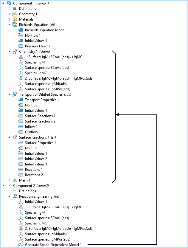
The model tree with the 2D model component with the Richard’s Equation Model, the Chemistry, Transport of Diluted Species, and the Surface Reactions interfaces, as well as the 0D model component with the Reaction Engineering interface. The Generate Space Dependent Model node adds the transport and chemistry interfaces to the already existing 2D model component with the Richards’ Equation interface.
The model tree is shown in the figure above for the IgM reaction path. The Chemistry, Transport of Diluted Species, and Surface Reactions interfaces are all created by the Reaction Engineering interface, where the chemical reactions are defined using the Generate Space-Dependent Model functionality.
The chemical reactions in the conjugate pad are defined as follows:
- The reaction between IgM and the SARS Co-2 antigen on the gold nanoparticle in the conjugation pad is defined as: IgM +SCoAu(ads) => IgMC
- The term (ads) is used to denote that the antigen and the nanoparticles are adsorbed in the pore structure of the conjugate pad and are picked up by IgM to form the complex IgMC, which is dissolved in the solution.
- We get the analogous reaction for the IgG antibody: IgG + SCoAu(ads) => IgGC
- The reaction of the animal antibody (AA) with the animal antigen on the gold nanoparticles (AAu) may be defined as: AA + AAu(ads) => AAC
IgMC, IgC, and AAC are thus the antibody–conjugate complexes.
The reactions in the test lines are as follows:
- In the first test line, we have: IgMC + IgMd(ads) => IgMPos(ads)
- Illustrating that the IgMC complex reacts with the adsorbed IgMd detector protein to form the adsorbed IgMPos surface species. The formation of the immobilized IgMPos gives the first test line its detection color.
- Analogously to 4 above, in the second test line we have: IgGC + IgGd(ads) => IgGPos(ads)
- The adsorbed species IgPos gives the second test line its red color.
- In the third test line, we thus have: AAC + AAd(ads) => AAPos(ads)
- The adsorbed species AAPos gives the control test line its red color.
The Model Results
The figure below shows the flow profile in the test strip at four different times. We can see that, initially, the sample fronts reach further into the test strip along the middle of the test strip, forming a slightly parabolic profile. The parabolic profile is due to the position of the sample well in the middle of the test strip. However, after 5 seconds, when the flow has already reached about one third into the conjugate pad, the flow profile is flat (see the last figure in the previous blog post).

The sample already reaches the first conjugate area after 3 seconds. Here, you can still notice the impact of the position of the sample well on the spreading of the sample, since it is not flat but shows a maximum reach in the middle. After 21 seconds, by the time the sample has reached the first test line area, the velocity profile is a straight line. After 65 seconds, the flow has reached the reference test line, and after 100 s it has reached the absorption pad.
We can also see in this plot that the solution is symmetric along a plane perpendicular to the test strip in the middle of the channel. This means that we could have solved the problem for only one half of the device. Modeling the whole device, despite the fact that the problem is symmetric, is a good way of checking that the mesh is dense enough to draw any conclusions on the flow profile. The fact that the flow profile is symmetric tells us that the mesh may be dense enough here.
Let us also look at the plot of the flow velocity of the sample at the position of the first test line; see the figure below. We can see that the flow starts at around 20 seconds after the sample has been applied to the sample well. The flow stops at around 275 seconds. This coincides with the time when the absorption pad becomes full with the liquid sample.
What is also interesting is that the flow rate decreases with time with an almost exponential decay. This is due to the fact that the capillary force that drives the flow acts only on the pore surfaces where the sample liquid meets air (the three-phase boundary area of the liquid front). This means that this force is constant, as long as there is free pore volume to fill up with sample liquid. However, the resistance to the flow increases as the sample liquid reaches further into the test strip. The pore wall area in contact with the flowing sample liquid increases with time and thus also the friction area between the pore walls and the flowing liquid.

The sample flow velocity at the position of the first test line for the 3D model (blue) and the 2D model (green). The two curves are in decent agreement. The 3D model shows a delay of about 2 seconds, which is probably due to the fact that the sample has to initially flow along the width. In the 2D model, the sample is instantly spread evenly along the width.
The concentration of the IgMC complex is shown in the figure below for different time steps. We can see that IgMC travels with the fluid flow until it reaches the area of the first test line. Here, it is consumed by the reaction with the IgM detection species to form the colored detection line. The IgMC concentration field shows that, after reaching the test line, a concentration boundary layer is formed. The concentration depletion plume after the test line continues to develop with time, but the area around the test line reaches almost a steady state. However, once the flow stops, when the absorption pad is saturated by the sample, then a thicker depletion area forms below the test line, which reaches all across the membrane. In similar fashion, the area beneath the conjugation line is saturated by the IgMC species.

The concentration field of IgMC as a function of time at the conjugation pad and in the membrane. The times are after 21 seconds (top), 65 seconds, 260 seconds, and 410 seconds (bottom). After 410 seconds, there is no longer any flow through the test strip. We get a zone with high IgMC concentration in the conjugate pad and a zone with low IgMC concentration below the test line for IgM.
The impact of the flow is clear if we plot the particle concentration of the detection species at the surface of the test line. The increase in particle concentrations starts with a delay given by when flow reaches the respective test line. The concentration grows almost linearly as IgMC is adsorbed at the test line area and the detector species IgMPos is formed. The linear increase means a constant adsorption rate. When the flow stops, due to the saturation of the absorption pad, the rate of formation of IgMPos continues about the same rate. This implies that, in this case, the formation of IgMPos is determined by the adsorption kinetics, i.e., it is determined by the adsorption rate of the gold nanoparticles in IgMC to the adsorption site. If it was mass transport controlled, we would see a change of the slope of the curve and the grow would be slowed down when the flow stops. This could, of course, change if we change the rate constant for the adsorption kinetics. The visibility of the test lines starts at about 1·108 particles/mm2.

The concentration of IgMPos, IgGPos, and AAPos at their respective test line surface as a function of time. IgMPos and IgGPos compete for the same conjugate label and therefore AAPos grows slightly faster.
So, if the kinetics is similar for the three test lines we would see a delay of the first, second, and third (control) test line revelation in that order. In addition, each test line would start to be colored at the edge facing the flow, with the trailing parts of the test lines revealed slightly later.
The homogeneous model shows similar results, if we tune the kinetics for the homogeneous case. However, here the transport is much faster, since the reaction sites are spread all across the thickness of the conjugate pad and, for the test line, across the membrane thickness. The reactants do not have to be transported to the surface of the test strip. This gives a more mixed process, where both kinetics and mass transport limit the revelation of the test line. The figure below shows the IgMC concentration corresponding to the heterogeneous case above.

The IgMC concentration for the case where the conjugate area contains the conjugate label across the whole thickness and the test line is present across the whole thickness of the membrane. The results are similar to the heterogeneous case.
The plot below shows the revelation of the test line. We can see that it starts to reveal almost uniformly with a small tilt in the the direction of the flow. When the flow stops, we get a higher color saturation on both edges of the test line, since there is higher transport of the antibody–conjugate complex by diffusion to these edges.

Concentration of IgMPos per unit surface area integrated over a thickness of 10 μm at the IgM test line. The plots are from 20 seconds to 400 seconds with 20 seconds increments. The curves start at 20 seconds at the bottom (low saturation) and end at 400 seconds at the top (high saturation). After around 260 seconds, the curves are closer between time steps, since diffusion is then the only way to transport the antibody-conjugate label complex to the test line area, thus slowing down the process.
The reality may be something in between the homogeneous and heterogeneous model. One can think that a good approach to get a test line that is colored uniformly across its width would be to have a detection volume close to the surface of the test strip. In this way, transport can occur from the x and y directions, and at the same time we get a relatively large reaction zone (see the figure below). Spreading the reaction zone across the whole thickness of the membrane, for the test line, does not contribute to the visibility of the test either, since the membrane is not transparent. However, it is an advantage if the reaction zone in the conjugate pad is distributed across the whole thickness, since this would maximize the reaction between the conjugate label and the antibody. In this way, the conjugate label would pick up as much antibodies as possible.

In this configuration, the test line’s reaction zone is not limited to the surface but is is not distributed across the whole thickness of the membrane either, it is limited to a thickness of 15 μm. The membrane is not transparent, but rather opaque with a visibility depth of around 10 μm. A limited test line thickness allows for a transport across the whole width of the test line thus yielding a relatively uniform color saturation across the width of the membrane.
Concluding Thoughts
The interval of sample flow over the test strip is determined by the size of the absorption pad, which also determines the size of the sample. This is obvious of course, and nothing new for scientists and engineers working with LFA devices. What is more interesting is that the model predicts the exponential decay in flow rate as the sample progresses over the test strip, which is also well known for scientists in the field, but maybe not completely obvious.
The 2D simulation shows that the mass transport in the test strip, in the heterogeneous case, seems to be slow, but the adsorption kinetics seem to be the rate-determining step anyway. The flow seems to quickly distribute the sample over the test strip. However, the adsorption reaction is so slow that it still limits the formation of the detection species at the test lines in the heterogeneous case. In the homogeneous case, the kinetics are even more limiting, since the transport to the reaction site is directly in the direction of the flow and does not have to rely on diffusion, at least as long as there is flow of the sample. However, these results are of course related to the input data that we have used.
The models created for this blog post are schematic in terms of the chemistry. In order to use them for real development of test strips, much larger efforts have to be made in the generation of the input data for the chemistry and for the properties of the porous materials. However, the models include the important phenomena: relatively detailed transport and reaction descriptions.
Possible Model Improvements
- Account for adsorption–desorption everywhere along the membrane: Here we assume that all species transport freely until they are permanently adsorbed at the test lines.
- More accurate two-phase flow model. We used a simple two-phase flow model for porous media. A more accurate model based on the phase field could also be used.
- Input data from a specific test published in scientific literature: We used the same porosity and wetting properties for all pads in the test strip assembly. The concentrations and adsorption kinetics use input data that generates reasonable results. However, a literature search should be done in order to use realistic data for the concentrations and kinetics. However, this would be different for different COVID-19 tests and every manufacturer has its own sample preparation and detection procedure. The purpose of this blog post is to present possible modeling approaches, not to publish a scientific paper.
- Mesh convergence analysis. This would show the accuracy that you can expect in the simulation results. This was partially done, and we know that the models give relatively small numerical error. But doing this in a strict way is outside of the scope of this blog post.
References
- L. Gutierrez, J. Beckford, and H. Alachkar, “Deciphering the TCR Repertoire to Solve the COVID-19 Mystery”, Trends in Pharmacological Sciences, vol. 41, no. 8, pp. 518–530, 2020, (https://www.cell.com/trends/pharmacological-sciences/fulltext/S0165-6147(20)30130-9),
- D. Rath and B. Toley, “Modelling-Guided Design of Paper Microfluidic Networks – A Case Study of Sequential Fluid Delivery”, ChemRxiv, 2020, https://doi.org/10.26434/chemrxiv.12696545.v1.
Download the Models
Ready to try modeling a rapid detection test for COVID-19? Access the model files by clicking the button below:


Comments (6)
Alex H
July 2, 2021Can the homogenous reaction be modeled using the porous packed bed automatically couple the flow without having to secondary ODEs?
Ed Fontes
July 2, 2021 COMSOL EmployeeHi Alex,
Yes you can. The problem with the packed bed is that it consists of microporous particles, where also a diffusion-reaction problem is solved along the radius of the particles in each point in space (an extra dimension). This is valid for systems with bimodal pore distribution with larger pores between particles and smaller pores inside the particles.
The membrane in the rapid test does not consist of such a pore structure. This is not a problem though, one could define almost solid particles and still use the ready-made packed bed feature. The drawback is that since we have to solve a diffusion-reaction problem in each point in space along the particle radius, performance is substantially lower than defining a simpler problem using ODEs. However, in the next release, we will include a feature for packed beds that do not consist of microrporous particles. This is a simpler problem so it is kind of silly that we did not include this until now. But I have to admit that I discovered that this simple case was not covered when I wrote the blog. That is when we decided to add this for the next release.
Best regards,
Ed
Alex H
July 2, 2021Very cool! Thank you for the speedy response. I was wondering why you did not use the porous packed bed and opted to use the self-defined system of ODEs.
I am trying to simulate something similar where antigens are immobilized on a 20 micron-thick porous substrate instead of a 2D surface with additional wash steps and reversible kinetics. I’ve found that setting the “Pellet-fluid surface” to “Continuous Concentration” provides similar results to the non-microporous particle. Good to know that the next release will help speed up my simulations!
Much thanks,
Alex
Sefan Maert
June 27, 2023I found this article really fascinating. As someone interested in the field of diagnostics, it’s great to see the application of simulation and modeling in developing efficient COVID-19 tests.
The article explains how these checks work by detecting IgM and IgG antibodies, which are produced by the immune device in response to a viral infection. The models discussed in the article provide insights into the distribution of sample liquid, flow dynamics, and the reactions occurring in the test strip.
I was particularly impressed by the 3D model’s ability to simulate the flow profile and the uniform distribution of the sample. It’s intriguing how the sample fluid forms a flat velocity profile along the width of the test strip, ensuring accurate test results. The 2D models further enhance our understanding of the transport and reactions within the test strip.
The concentration plots for the IgMC complex showcase the dynamic behavior of the test. It’s fascinating to observe how the complex travels with the fluid flow, reacts at the test lines, and forms the colored detection lines. Additionally, the insights gained from studying the flow velocity and the saturation of the absorption pad provide valuable information for optimizing the test design.
Maria Pereira
July 3, 2025I’m trying to simulate a lateral flow in COMSOL but I don´t know how can I design the control line and test line. In the part of the chemistry, for me doesn’t appearance the surface species. Can you help me please ?
Ed Fontes
July 4, 2025 COMSOL EmployeeDear Maria,
To help the Chemistry interface recognize that you’re defining a surface species or a surface reaction, you need to add (ads) after the species name in the Formula field of the Reaction settings window. Here’s a simple example you can try:
1. Right-click the Chemistry node and select Reaction from the context menu.
2. Select the newly created Reaction node.
3. In the settings window for Reaction, enter IgM => IgM(ads) in the Formula field, then click Apply.
After this, the reaction feature should be interpreted as a Surface feature, and IgM(ads) will be defined as a Surface species.
Best regards,
Ed