

With the release of version 6.2 of the COMSOL Multiphysics® software, electrical dispersion modeling capabilities can now be extended to the Electric Currents interface, which supports both time- and frequency-domain modeling. This functionality is especially important for the accurate modeling of a wide class of materials, including insulators and living tissue. Let’s briefly review what dispersion is, and then we’ll show how to include it in your COMSOL models and discuss why it is important.
Background
Whenever modeling fast pulses of electric current applied to living tissue, such as in the context of cardiac ablation, electroporation, or neural stimulation, the dispersive nature of the tissue, as well as the electrical insulators, needs to be considered.
All materials are electrically dispersive, meaning that relative permittivity varies with the frequency of excitation. Permittivity is a measure of how a material will respond, or polarize, in the presence of an electric field. The magnitude of this response varies with frequency due to the different atoms and molecules within the material and their structure. It is also a measure of how much electric energy is converted into heat, or lost, when the material is exposed to a time-varying signal. These losses arise because of the relative motion of the atoms and molecules as they oscillate in the time-varying fields. When working in the frequency domain, the relative permittivity is expressed as a complex-valued number: \epsilon_r =\epsilon_r^{‘}- i \epsilon_r^{”}, where the real and imaginary components are related via the Kramers–Kronig relations. Two such dispersion curves are shown in the figure below, representing an insulative material and living tissue, respectively. The former has a relatively simple curve, with almost uniform properties over a wide frequency band, so we can see that it is not always necessary to consider dispersion. On the other hand, there will always be a frequency band over which there are significant variations in properties and it is necessary to consider dispersion.

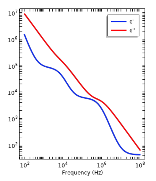
Representative dispersion curves of an insulator (left) and human tissue (right). The magnitude of the real- and imaginary-valued component of the relative permittivity are plotted.
In addition to these frequency-dependent losses, there are also electrical losses in a static electric field, and these are quantified by the DC electric conductivity, \sigma_{DC}. All materials have some DC conductivity, but it can be very, very small. This is a separate loss mechanism from the dispersive loss. It can be convenient to express all of the material losses, regardless of mechanism, via the total conductivity: \sigma_{tot} =\sigma_{DC} + 2\pi f \epsilon_0\epsilon_r^{”}, and this is plotted below for the same two materials. It is important to remark, however, that frequency-dependent conductivity can also be presented without the DC component as \sigma(f) = 2\pi f \epsilon_0\epsilon_r^{”} with \sigma_{DC} reported separately.
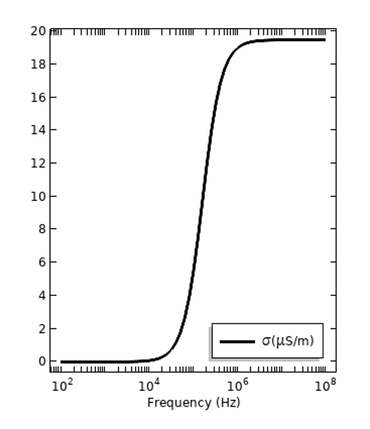
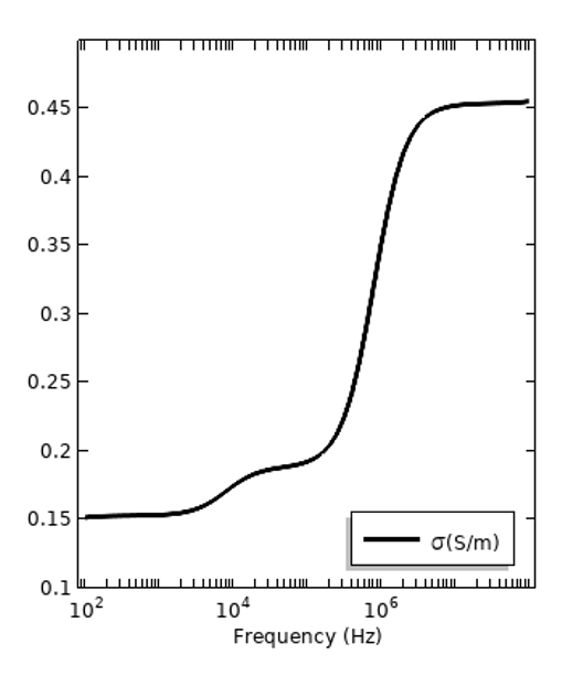
The losses of the same two materials in terms of total electric conductivity, with the DC conductivity presented in contribution to the dispersive loss.
Although material properties are experimentally determined, we don’t want to use the experimental data directly since it will have some uncertainty to it and will not satisfy the Kramers–Kronig relations, thus leading to a noncausal model. Instead, we fit to the data a function that already satisfies that Kramers–Kronig relations and use the coefficients of that fitted function to describe our material behavior. Currently, the software supports the Multipole Debye model, which takes as input any number, N, of poles, where each pole, m, has a relaxation time, \tau_m, and relative permittivity contributions, \Delta \epsilon_r_m, and from these defines the complex-valued permittivity as:
where \epsilon_\infty is based on either the low-frequency limit, \epsilon_\infty \rightarrow \epsilon_{rS}-\Sigma \Delta \epsilon_r_m, or the high-frequency limit, \epsilon_\infty \rightarrow \epsilon_{rS}. In addition, the relaxation times can optionally be shifted due to a change in temperature using any one of the Vogel-Fulcher, Arrhenius, Williams-Landel-Ferry, or Tool-Narayanaswamy-Moynihan shift functions, or even a user-defined shift function.
If you instead have experimental data for the real and imaginary components of the permittivity and want to fit a Debye model to that, this can be done with the Partial Fraction Fit functionality in COMSOL® version 6.2. For a guide to using this functionality, see our Learning Center article “Fitting the Debye Dispersion Model to Experimental Data”.
Using the Electric Currents Interface
Including dispersion in an Electric Currents model requires only a few steps. First, a Current Conservation domain feature has to be added and applied to the relevant domains. Within that feature, the Material Type has to be set to Solid. This can still be used to model a fluid, under the assumption that the fluid is not deforming.
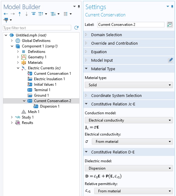
The Current Conservation feature, where the Dispersion dielectric model can be selected.
After changing the Dielectric model option to Dispersion, an additional subfeature will appear. Within this feature, the branches of the Multipole Debye model are entered as well as the limiting behavior, as shown in the screenshot below. As an alternative to entering the poles, or branches, it is also possible to specify the relaxation data via the Constant Loss Tangent model, which takes a loss tangent, center frequency, and bandwidth as input. From these inputs, the software will automatically determine the number of poles, relaxation times, and relative permittivity contributions. It is also possible to use the simpler Debye model, which has a single pole. The thermal effects that cause a shift in the relaxation times can optionally be enabled with the Thermal Effects settings.
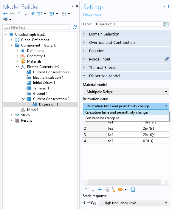
The Dispersion subfeature, where the branches of the Multipole Debye model are entered and the limiting behavior is specified.
Looking at Results
We can look at how dispersion affects the response of a simple system, such as a parallel plate capacitor operating in the frequency domain and try out our two different materials sandwiched inside. We can see from the plots below how the real and imaginary components of the impedance vary with frequency.
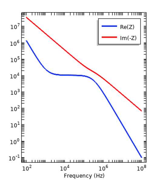
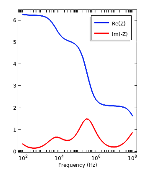
Impedance of a parallel plate capacitor with a sample of an insulator (left) and tissue (right) inside. Note that the negative imaginary component of the impedance is plotted.
We can also use the same model to look at the results of a time-domain excitation of the same system. We will look at solely the sample tissue material, since the variation in response over frequency is more dramatic. The setup of the dispersive material is the same, but it is worth reviewing the various ways of exciting such a system. We begin by exciting the system with a smoothed step in the applied current, ramping from 0-1A over 10 ns, and computing the response over 100 µs by plotting the voltage sensed at the terminal (see figure below). Results are plotted over time, and over time in log scale.
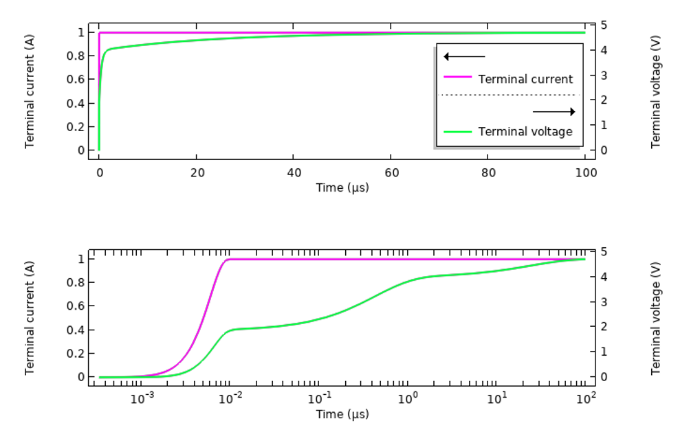
The transient response of the sample tissue material with an imposed current over time.
It is interesting to contrast these results with a model excited via a similarly smooth stepped voltage signal propagating along a transmission line. The figures below show the response in terms of measured current and voltage. Note that the voltage signal plotted here is the sum of the incident smoothed step voltage signal and the reflected signal from the structure and the material. This total signal exhibits time-varying behavior due to the dispersive material.
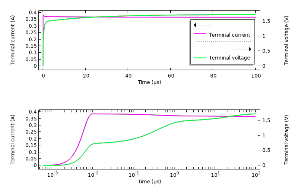
The transient response of the sample tissue material excited via a transmission line, with a stepped voltage signal.
Closing Remarks
Modeling of electrical dispersion within the Electric Currents interface is now possible and easy to set up. This material model gives a more accurate picture of the true electrical response as well as the losses in both frequency- and time-domain models. This functionality is useful for the modeling of many materials.
It is worth remarking that electrical dispersion modeling is also possible via the Electrostatics interface and has been since version 6.0, in which it is intended primarily for the purpose of modeling lossy piezoelectric materials. In addition, if modeling at much higher frequencies, the RF Module and the Wave Optics Module include other dispersion models.

Comments (0)