
As of version 6.0 of the COMSOL Multiphysics® software, there is a convenient feature for modeling applications involving the use of piezoelectric devices. The Piezoelectric Waves, Time Explicit interface extends the existing discontinuous Galerkin (dG or dG-FEM) method for acoustics in fluids and linear elastic materials to piezoelectric media. This makes it an efficient alternative to model the generation and reception of sound waves that travel over large distances relative to the wavelength. Applications that can benefit from this feature include ultrasound imaging, nondestructive testing (NDT), flowmeters, and interdigitated surface acoustic wave devices, etc. Let’s take a closer look at this feature.
About the Piezoelectric Waves, Time Explicit Interface
The Piezoelectric Waves, Time Explicit multiphysics interface can be found under the Acoustics > Elastic Waves branch, and is available for 2D, 2D axisymmetric, and 3D analyses.
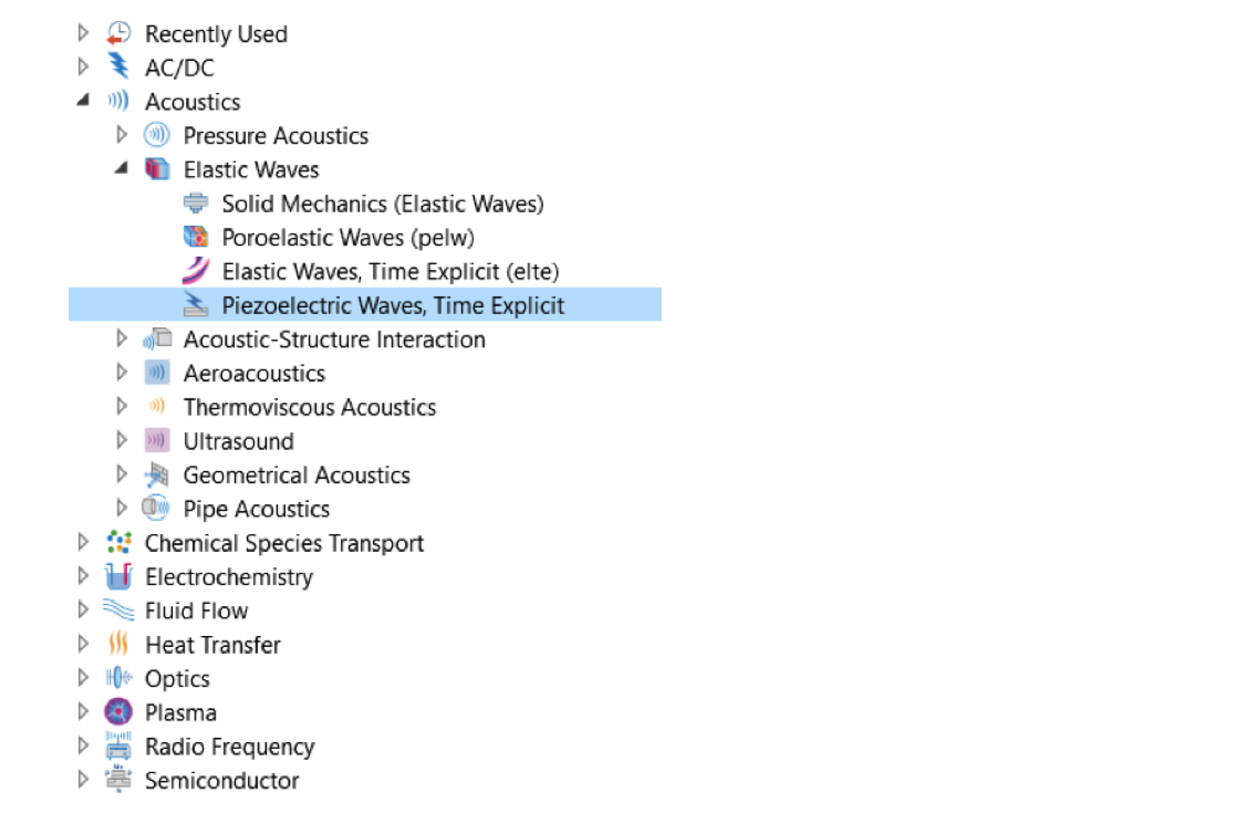
How to access the new interface from the Add Physics wizard.
Both the direct and inverse piezoelectric effects can be modeled and the piezoelectric coupling can be formulated using the strain-charge or stress-charge forms. Therefore, it is suited for large, transient acoustic problems when piezoelectric devices are used as either transmitters, receivers, or both at the same time. This multiphysics interface combines the Elastic Waves, Time Explicit interface and the Electrostatics interface together with the new Piezoelectric Effect, Time Explicit multiphysics coupling. The elastic waves problem is implemented using the higher-order dG formulation and is solved with a time-explicit solver, while the electrostatics problem is solved at every time step through an algebraic system of equations implemented with the finite element method (FEM). This allows the fully coupled problem to be solved with an explicit time-stepping method, and only the electrostatic equations are solved with a matrix-based method. In all, this constitutes a memory efficient method that is also well suited for distributed computing on clusters.
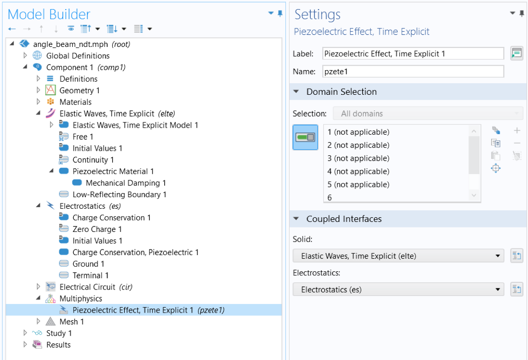
User interface for the Piezoelectric Waves, Time Explicit interface, here shown with the Angle Beam Nondestructive Testing tutorial model.
When adding the Piezoelectric Waves, Time Explicit multiphysics interface, two material models are included in each physics to account for the constitutive relationships in different materials. The Elastic Waves, Time Explicit physics contains an Elastic Waves, Time Explicit Model material node for linear elastic materials and a Piezoelectric Material node dedicated to piezoelectric domains.
Rayleigh damping can be applied to both material models to include mechanical loss. In parallel, the Electrostatics physics interface contains a Charge Conservation material node for regular dielectric materials and a Charge Conservation, Piezoelectric node for piezoelectric domains. The former supports conduction loss, while the latter supports dispersion models to capture dielectric loss. The two piezoelectric material models in the two physics are then coupled through the Piezoelectric Effect, Time Explicit multiphysics feature.
Using Form Assembly and Identity Pairs
As explained in the “Meshing and Solving” section in the “Introduction to the Elastic Waves, Time Explicit Interface” blog post, it is important to use a nonconforming mesh with an assembly geometry when coupling domains with different properties, which is almost always true for applications involving piezoelectric devices. In short, this is to avoid small internal solver time steps due to unnecessarily small mesh elements in a specific material domain; the time step depends on local mesh size and speed of sound, also known as the cell wave time scale.
As you can see in the image below of the Angle Beam Nondestructive Testing tutorial model, we use different mesh sizes to discretize solid domains with different material properties, and the meshes are nonconforming at the material interfaces. It is recommended to always use imprints for assemblies to increase both performance and stability. Our blog post on “Introduction to the Elastic Waves, Time Explicit Interface” shares a detailed discussion on the general guidelines on meshing and solving dG-based physics.
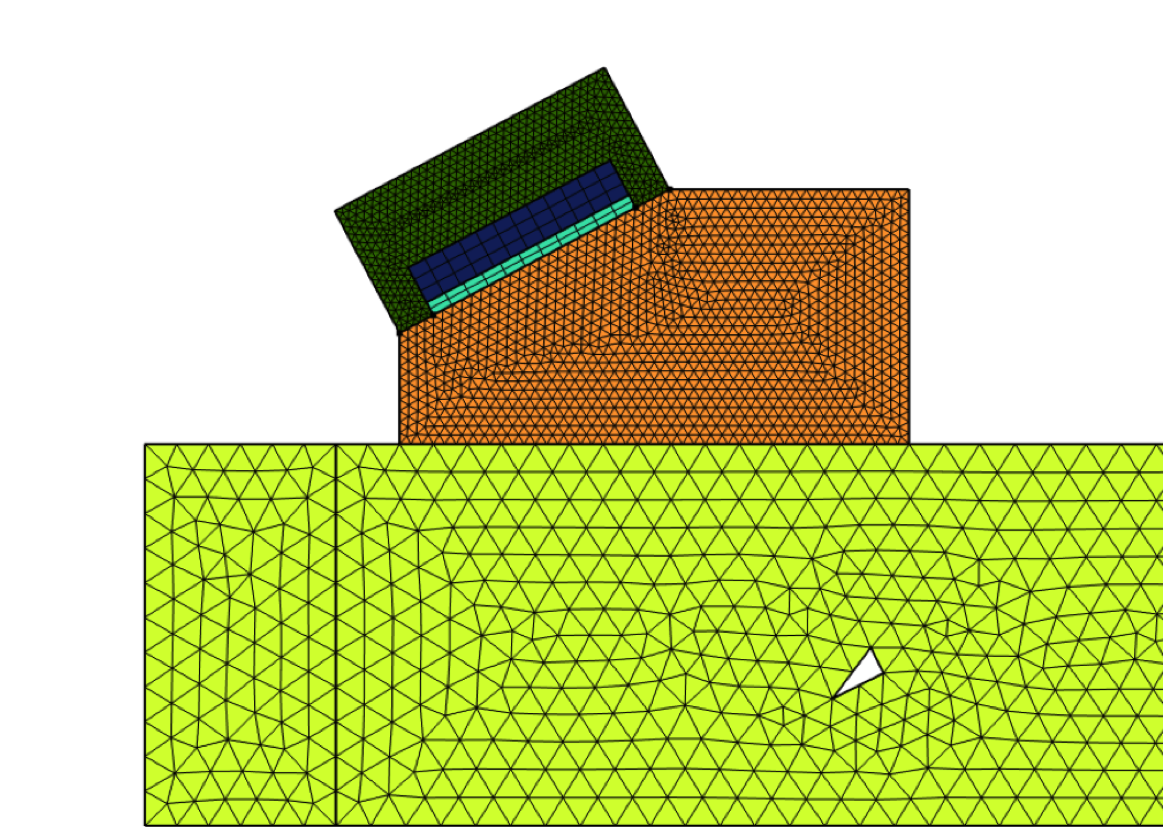
A close look at the nonconforming mesh used in the Angle Beam Nondestructive Testing tutorial model. Different colors indicate different materials.
COMSOL Multiphysics version 6.0 makes it more convenient for you to set up the model using nonconforming meshes. When the geometry parts are connected via form assembly and the identity pairs are created, a Continuity node is automatically added to the Elastic Waves, Time Explicit physics with all Identity Boundary Pairs selected (as shown below). This ensures continuity in velocity and normal stress, and so all phenomena occurring at the material discontinuous interfaces are simulated.
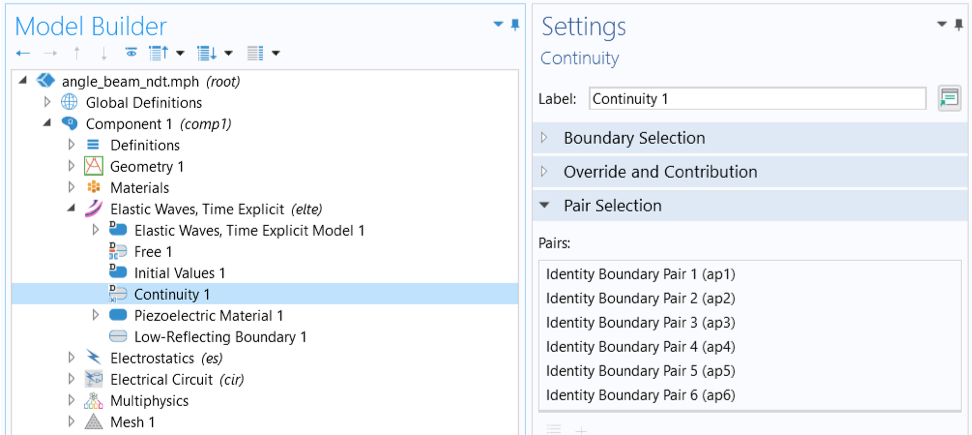
A Continuity node is automatically added to the Elastic Waves, Time Explicit physics interface for an assembled geometry.
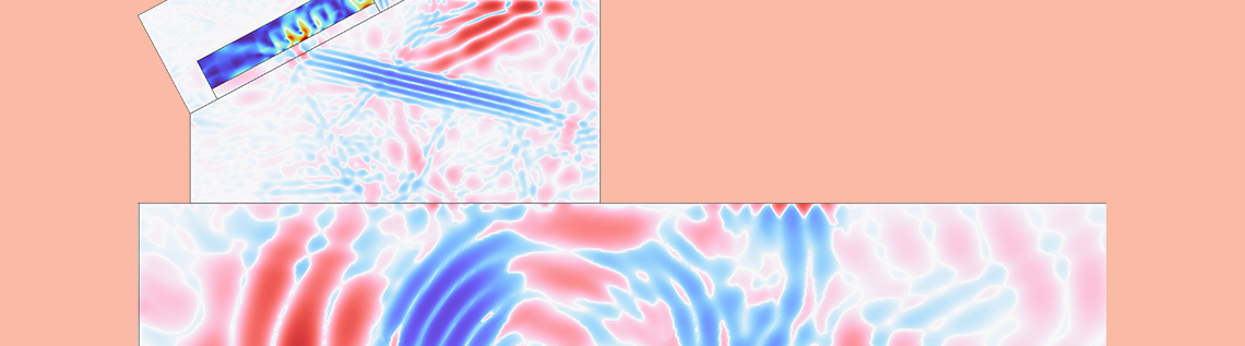
The animation below shows the conversion of a longitudinal (compression) wave sent by the transducer into a refracted shear (transverse) wave when the signal hits the surface of the test sample. The longitudinal waves are shown in blue and shear waves in orange. The shear wave is then reflected by the flaws in the test object, transmitted back, and picked up by the transducer. This is the operating principle of angle beam NDT, as shear waves have lower attenuation and shorter wavelength, which makes them capable of detecting smaller defects.
The Angle Beam Nondestructive Testing tutorial model showing wave refraction and reflection at the material interfaces.
Postprocessing
The most important thing to keep in mind when postprocessing is that the dependent variables are discretized by fourth-order elements. We can view the spatial details contained within each mesh element by setting a high resolution in the Quality section for the plots.
The cell wave time scale variable, elte.wtc, is now available directly in postprocessing, along with the minimum cell wave time scale variable, elte.wtcMin, which gives the global minimum value. The cell wave time scale is directly related to the solver time step; therefore, an examination of its value can help identify problematic mesh elements in the model. When plotting this variable, set the Resolution field to No refinement and the Smoothing field to None. Both settings can be found in the Quality section of the plot.
Note: Additional tips for postprocessing results from the time-explicit interfaces are discussed in the “Introduction to the Elastic Waves, Time Explicit Interface” blog post.
Coupling with dG-Based Pressure Acoustics Interfaces
When the sound propagation path includes fluids, you can add either a:
- Pressure Acoustics, Time Explicit interface for linear wave propagation in the fluid domains, or
- Nonlinear Pressure Acoustics, Time Explicit interface for capturing higher harmonics generation as waves travel through fluids.
Either of these interfaces can be coupled to the Elastic Waves, Time Explicit interface using the built-in acoustic–structure coupling features. There are two versions of the coupling: an Acoustic-Structure Boundary, Time Explicit coupling for geometries that have solid and fluid parts unioned and discretized with a conforming mesh, and a Pair Acoustic-Structure Boundary, Time Explicit coupling for assembled geometries using nonconforming mesh. The pair coupling feature can be more advantageous in acoustic–structure interaction analyses due to the vast property differences between solids and fluids. An example is the Ultrasonic Flowmeter with Piezoelectric Transducers tutorial. The model uses the pair coupling feature at the transducer–water interfaces to capture sound transmission and reflection happening at the material discontinuity.

The Pair Acoustic-Structure Boundary, Time Explicit coupling is used in the Ultrasonic Flowmeter with Piezoelectric Transducers tutorial model.
Try It Yourself
- You can see how the Piezoelectric Waves, Time Explicit interface is used in the following models:
- Further reading:


Comments (6)
Daniel Oliveira
February 9, 2022Excellent explanation Jinlan Huang, thannk you!
To differentiate the longitudinal waves from shear waves you use the expression “sqrt(abs(elte.I2s))*sign(elte.I2s)”, I thought that it only serve for isotropic materials, would you have any suggestion for anisotropic materials?
Jinlan Huang
February 11, 2022 COMSOL EmployeeHi Daniel, we would suggest using this expression for isotropic materials only. In general, we cannot tell about pure pressure and shear waves for anisotropic materials; rather quasi-longitudinal and quasi-shear waves, as shown in the Isotropic-Anisotropic Sample: Elastic Wave Propagation tutorial example (https://www.comsol.com/model/isotropic-anisotropic-sample-elastic-wave-propagation-78231). We are aware of publications on the p- and s-waves separation – not for anisotropic but at least for transverse isotropic materials – but those algorithms have not been implemented and tested in COMSOL.
Daniel Oliveira
February 16, 2022Thank you Jinlan for the posts and the excellent video tutorials!
Ahmed Hassan
November 7, 2023Could you please help me how to generate wave signals with defects and without defects for the Angle Beam Nondestructive Testing tutorial model showing wave refraction and reflection at the material interfaces?
Or any references that would help to learn how to generate reference signals and detect defect signals.
Jinlan Huang
November 8, 2023 COMSOL EmployeeHi Ahmed, for a system when there is no analytical solution available, you will need to solve the model without including the defect to get the reference signal. Use the angle beam ndt tutorial as an example, you remove the Fracture node to compute for the reference solution.
Ahmed Hassan
November 8, 2023the tutorial didn’t show the steps in how to generate the reflection signal.