
Almost all media absorb electromagnetic radiation to some extent. In high-powered laser focusing systems, a medium such as a glass lens may absorb enough energy from the laser to heat up significantly, resulting in thermal deformation and changing the material’s refractive index. These perturbations, in turn, can change the way the laser propagates. With the Ray Optics Module, it is possible to create a fully self-consistent model of laser propagation that includes thermal and structural effects.
Fundamentals of Thermal Lensing
To understand how ray trajectories are affected by self-induced temperature changes, consider a collimated beam that strikes a pane of glass at normal incidence. Assume that an antireflective coating has been applied to the glass surface so that the rays are not reflected. A typical pane of glass absorbs a very small, but nonzero, fraction of the power transmitted by the beam. If the power is sufficiently low, the temperature change within the glass will be negligible, and the outgoing rays will be parallel to the incoming rays.
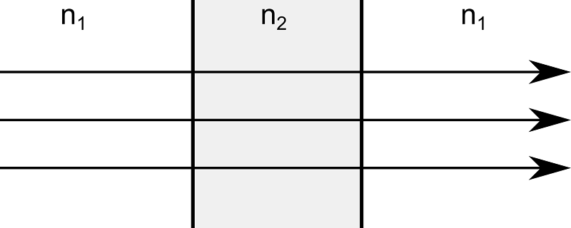
However, if a large amount of power is transmitted by the beam, the power absorbed by the pane of glass may substantially alter the temperature of the glass. The glass expands slightly, changing the angle of incidence of the rays and causing the transmitted rays to be deflected from their initially parallel trajectories. In addition, many materials have temperature-dependent refractive indices, and the temperature-induced change in the refractive index can also perturb the ray trajectories. Because the structural deformation and the change in refractive index tend to focus the outgoing rays, this phenomenon is known as thermal lensing.
Next, we take a more in-depth look at an application in which thermal and structural effects can significantly perturb ray trajectories.
Modeling a Laser Focusing System
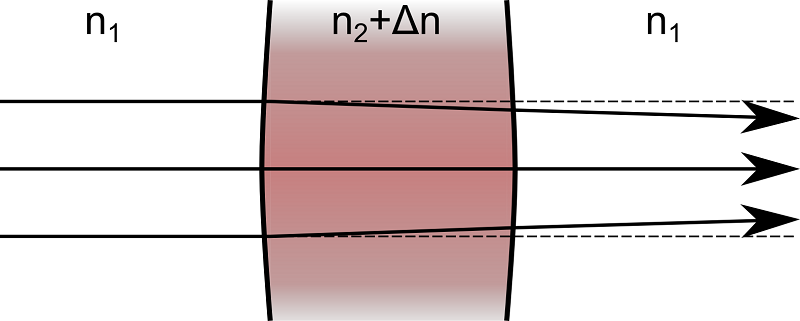
Consider a basic laser focusing system that consists of two plano-convex lenses. The first lens collimates the output of an optical fiber while the second lens focuses the collimated beam toward a small target.
If the laser beam delivers a small amount of power, then it is straightforward to model the propagation of the beam toward the target by using the Geometrical Optics interface and ignoring the temperature change in the lenses. The following image shows the trajectories of the rays in the lens system.
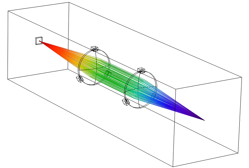
However, even a high-quality glass lens absorbs a small fraction of the electromagnetic radiation that passes through it. If the optical fiber delivers a very large amount of power, then a thermally induced focal shift may occur; in other words, the changes in refractive index and lens shape can move the focus of the beam by a significant amount. If it is necessary to focus the laser accurately, then the possibility of thermally induced focal shift must be taken into account when designing the lens system.
In this example, we will observe how the temperature change in the lenses causes the beam to be focused at a location several millimeters away from the target.
Modeling Ray Propagation in Absorbing Media
To model ray propagation in the thermally deformed lens system, we use the following physics interfaces:
- Geometrical Optics — To compute the ray trajectories.
- Heat Transfer in Solids — To compute the temperature in the lenses.
- Solid Mechanics — To model the thermal expansion of the lenses.
- Moving Mesh — To deform the finite element mesh in domains adjacent to the lenses.
The physics interfaces and nodes used in this model are shown in the following screenshot.
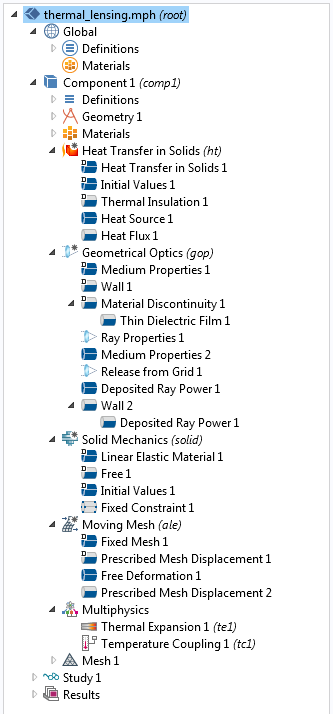
In addition to the Ray Optics Module, either the Structural Mechanics Module or the MEMS Module is needed to model the thermal expansion of the lenses.
Ray Trajectory Computation
Under the hood, the Ray Optics Module computes the ray trajectories by solving a set of coupled first-order ordinary differential equations,
(1)
\frac{d\mathbf{q}}{dt} &= \frac{\partial \omega}{\partial \mathbf{k}}\\
\frac{d\mathbf{k}}{dt} &= -\frac{\partial \omega}{\partial \mathbf{q}}
\end{aligned}
where \mathbf{q} is the ray position, \mathbf{k} is the wave vector, and \omega is the angular frequency. The wave vector and angular frequency are related by
(2)
where c is the speed of light in a vacuum. In an absorbing medium, the refractive index can be expressed as n-i\kappa, in which n and \kappa are real-valued quantities.
As the rays enter and leave the lenses, they undergo refraction according to Snell’s Law,
(3)
where \theta_1 and \theta_2 are the angle of incidence and the angle of refraction, respectively.
The intensity and power of the refracted rays are computed using the Fresnel Equations. In most industrial laser focusing systems, an antireflective coating is applied to the surfaces of the lenses to prevent large amounts of radiation from being reflected.
In this example, the antireflective coating is modeled by applying a Thin Dielectric Film node to the surfaces of the lenses.
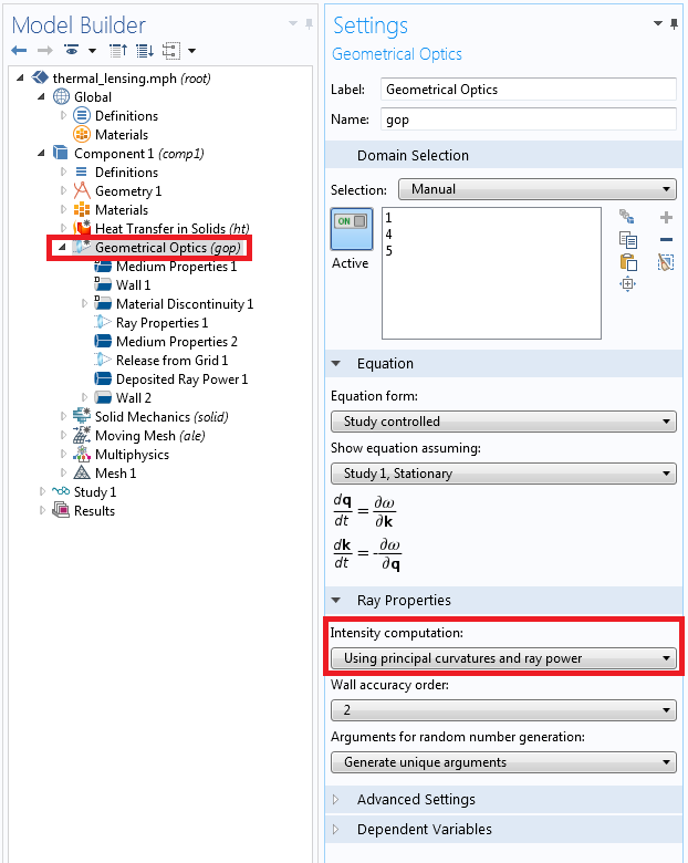
Computing the Power Transmitted by Each Ray
The variables that are used to compute ray intensity are controlled by the “Intensity computation” combobox in the settings window for the Geometrical Optics interface. To compute a heat source using the energy lost by the rays, select “Using principal curvatures and ray power”.
The total power transmitted by each ray, Q, remains constant in non-absorbing domains. In a homogeneous, absorbing domain, the power decays exponentially,
(4)
where k_0 is the free-space wave number of the ray.
In order to apply the power lost by the rays as a source term in the Heat Transfer in Solids interface, it is necessary to add a Deposited Ray Power node to the absorbing domains. This node defines a variable Q_{\textrm{src}} (SI unit: W/m^3) for the volumetric heat source due to ray attenuation in the selected domains. As the rays propagate through the lenses, they contribute to the value of Q_{\textrm{src}},
(5)
where Q_{j} (SI unit: W) is the power transmitted by the ray with index j, N_t is the total number of rays, and \delta is the Dirac delta function. In practice, each ray cannot generate a heat source term at its precise location because the rays occupy infinitesimally small points in space, whereas the underlying mesh elements have finite size, so the power lost by each ray is uniformly distributed over the mesh element the ray is currently in.
The following short animation illustrates how the heat source defined on domain mesh elements (top) is increased as the power transmitted by each ray (bottom) is reduced.
Computing the Temperature
The temperature in the lens, T, can be computed by solving the heat equation,
(6)
where k is the thermal conductivity of the medium. A Heat Flux node is used to apply convective cooling at all boundaries that are exposed to the surrounding air,
(7)
Structural Deformation
As the temperature changes, it contributes a thermal strain term \epsilon_{\textrm{th}} to the total inelastic strain in the lenses. The thermal strain is defined as
(8)
where \alpha is the thermal expansion coefficient, T is the temperature of the medium, and T_{\textrm{ref}} is the reference temperature. The resulting displacement field \mathbf{u} is then computed by the Solid Mechanics interface.
Obtaining a Self-Consistent Solution
If the power transmitted by the beam is very low, then the energy lost by the rays to their surroundings does not noticeably change the temperature of the medium. However, it is still possible for other phenomena, such as external forces and heat sources, to change the shape or temperature of the lenses.
In this case, it is necessary to first compute the displacement field and temperature in the domain, and then compute the ray trajectories. This is considered a unidirectional, or one-way, coupling because the temperature change and structural deformation can affect the ray trajectories, but not the other way around.
If the power transmitted by the beam is sufficiently large, then the dissipation of energy in an absorbing medium may generate enough heat to noticeably change the shape of the domain or the refractive index in the medium. In this case, the ray trajectories affect variables, such as temperature, that are defined on the surrounding domain, and these variables in turn affect the ray trajectories. This is considered a bidirectional, or two-way, coupling.
In this example, we assume that the laser is operating at constant power, so it is preferable to compute the temperature and displacement field using a Stationary study step. However, the ray trajectories are computed in the time domain.
To set up a bidirectional coupling between the ray trajectories and the temperature and displacement fields, we first create a Stationary study step to model the heating and deformation of the lenses, then add a Ray Tracing study step to compute the ray trajectories. Then, the corresponding solvers are enclosed within a loop using the For and End For nodes. The following image shows the solver sequence that is used to set up a bidirectional coupling between the ray trajectories and the temperature and displacement fields.
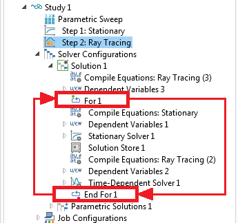
The nodes between the For and End For nodes are repeated a number of times that is specified in the settings window for the For node. Furthermore, every time a solver is run, it uses the solution from the previous solver. In this way, it is possible to set up a bidirectional coupling between the two studies and iterate between them until a self-consistent solution is reached.
Results of Our Thermal Lensing Model
We now examine the ray trajectories close to the target for two cases: A 1-watt beam and a 3,000-watt beam.
For the 1-watt beam, we observe that the focal point of the beam is extremely close to the target surface. The rays do not converge to a single point due to spherical aberration. For the 3,000-watt beam, we see that the beam has already started to diverge by the time it reaches the target surface. The following image compares the deposited ray power at the target for the two cases.
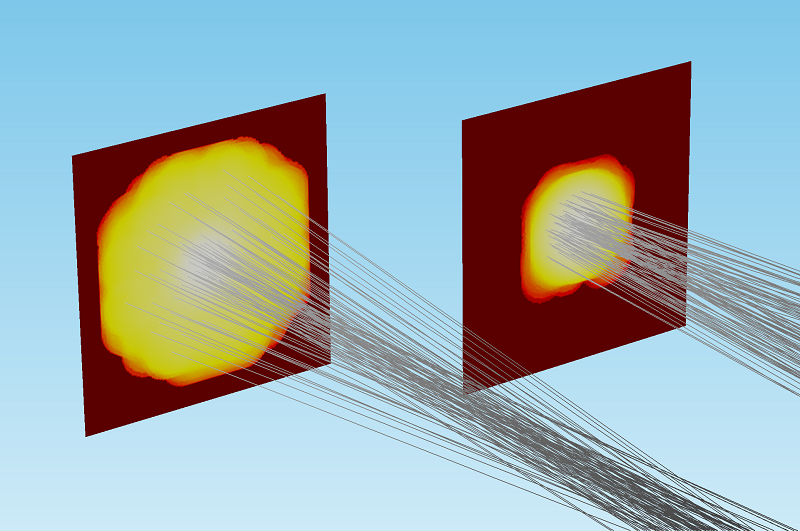
Comparison of the deposited ray power for a 3,000-watt beam (left) and 1-watt beam (right). For comparison and visualization purposes, the color expression for deposited power has been normalized and plotted on a logarithmic scale.
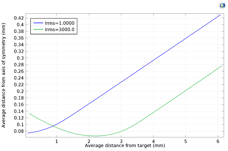
The Geometrical Optics interface also includes built-in operators for evaluating the sum, average, maximum, or minimum of an expression over all rays. Using these operators, it is possible to quantify the beam width in a variety of ways. As shown in the plot below, the 3,000-watt beam is focused more than 2 millimeters away from the target surface.
We have seen that the temperature change and the resulting thermal expansion in a high-powered laser system can significantly shift the focal point of the beam. With the Ray Optics Module, it is possible to take thermally induced focal shift into account when designing such systems.
Model Download
To learn more about computing ray trajectories in thermally deformed lens systems, please refer to the Thermal Lensing in High-Power Laser Focusing Systems model.


Comments (2)
Victoria Leoni
April 22, 2016mona aghaee
January 29, 2018Hi,
I have problem modeling radiation heat transfer in a slab. A constant radiation hits an slab and part of that is transferred through the slab, part is absorbed within the slab and part is reflected. How should I model this? I already know the absorptance, reflectance and transmittance coefficients of the slab. Please advise.
Thanks
Mona