

In outer space and other harsh radiation environments, high-energy ions and protons pierce materials and affect nearby electronic systems. Known as a single-event effect (SEE), the particle radiation can lead to soft or hard errors in devices. Since just one hard error puts a space mission at risk, aerospace engineers must make sure that all critical electronic devices can withstand an SEE. To gain a better understanding of this phenomenon, they can accurately analyze the ion-material interaction using simulation.
What Is a Single-Event Effect?
An SEE is an electrical disturbance in a circuit caused by charged particles, such as high-energy protons, hitting a solid material. The impact of these particles — which come from the Sun, radiation belts, and galactic cosmic rays — creates holes, enabling electrons to travel through the material. While moving, these free-charge carriers eventually recombine before stopping on a node. There, the extra charge causes a change in voltage and, in turn, a soft or hard error. These errors are particularly problematic for aerospace applications, although they can also occur on Earth in areas with high levels of radiation, such as near nuclear testing sites.
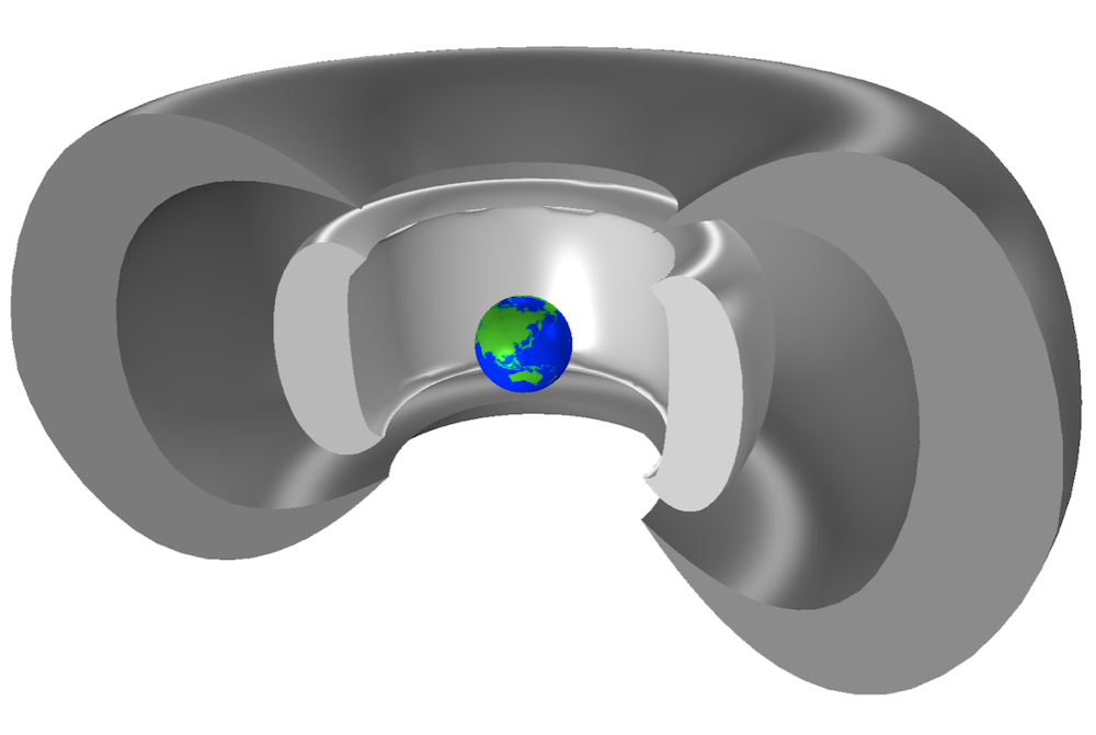
The charged particles in the Van Allen belts, which surround Earth for thousands of miles, could cause an SEE in a spaceship. The projection of Earth’s landmass is based on images by M.J. Brodzik and K.W. Knowles (Ref. 1).
Soft vs. Hard Errors
If just one hard error happens in a critical system in space, it could spell the end of the mission. For instance, the highly energetic particles produced by the 2003 Halloween solar storm affected numerous devices aboard spacecraft, including the Martian Radiation Environment Experiment (MARIE), which malfunctioned and never recovered. The reason is that hard errors can be destructive, sometimes to the point where the entire device or system needs to be replaced. Thankfully, though, not all errors caused by SEEs are so damaging. Soft errors typically aren’t destructive and can be fixed with a power reset.
An example of a soft error is a single-event upset, which occurs in two key components of digital electronic devices: memory and logic systems. These systems are integral to microprocessors, such as those in motherboards and scientific instruments on spacecraft. An error in the microprocessor could lead to the entire device behaving incorrectly simply by causing a bit to flip from a 0 to a 1 or vice versa. With this type of soft error, the system is usually able to keep functioning, and the issue can be fixed by reversing the change.
Hard errors, which include single-event latchups, burnouts, and gate ruptures, lead to more permanent effects. For instance, a single-event latchup can result in an operating current that is too high, causing the device to stop working properly; data to be lost; and ultimately, the device’s destruction. These latchups often take place in integrated circuits built with complementary metal-oxide-semiconductor (CMOS) technology, which is commonly used for microcontrollers and microprocessors. Burnouts and gate ruptures take place in, for example, power MOSFETs, such as those for weather satellites and GPS. These errors lead to voltages exceeding limitations, making the device fail.
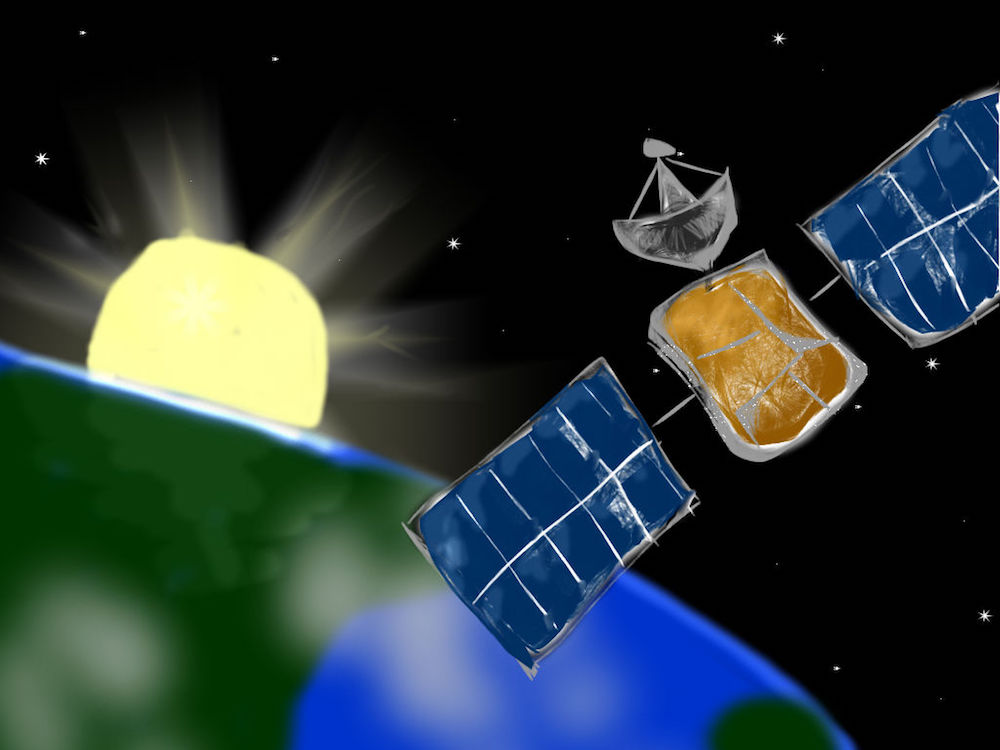
Hard errors in satellites can cause data to be lost and eventually lead to systems being destroyed.
Aerospace engineers must make sure that all important electronic devices avoid both soft and hard errors. This mission is becoming more of a challenge, though, due to the ever-increasing demand for technology with more functionality, smaller sizes, faster speeds, and lower voltages. While advantageous in terms of cost and performance, these factors mean that the critical charge (the minimum charge needed to upset a node) is getting smaller. As a result, lower-energy particles have a higher chance of causing SEEs, making devices more vulnerable to errors — even here on Earth.
By understanding how charged particles affect a material, aerospace engineers can design electronic equipment that can withstand, or even is invulnerable to, SEEs. To examine this interaction, they can use the COMSOL Multiphysics® software and add-on Particle Tracing Module, as demonstrated by a benchmark example.
Modeling Particle-Material Interaction with the COMSOL® Software
In this example, high-energy protons move toward a block of solid silicon for initial energy values ranging from 1 keV to 100 MeV. Once they hit the material, the protons undergo ionization losses, which slow the particles down, and nuclear stopping, which deflects them in random directions.
To easily capture the proton behavior, you can take advantage of the Charged Particle Tracing interface. Using the Particle-Matter Interaction node, you can account for both the energy loss as well as how the protons scatter. In addition, you can describe the effect of the proton on the material using one of the subnodes. For instance, the Ionization Loss subnode treats the interaction as a continuous force moving in the opposite direction of the particle’s motion, while the Nuclear Stopping subnode treats it as a discrete force slowing down the particle and deflecting it in a random direction.
Next, it’s important to determine the penetration depth of the particles (i.e., the ion range), as this influences whether or not they will ionize nearby electronic devices and thus cause an SEE. To find this depth, there are two approaches you can use:
- Using an auxiliary dependent variable to mimic the continuous slowing down approximation (CSDA), which assumes that the protons will slow down at a steady rate
- Computing the projected range by projecting the proton’s velocity onto its original direction of motion
Next up, you can see how these approaches compare to results from published literature.
Comparing the Simulation and Experimental Results
The protons tend to move in random directions at lower energies, as they’re more affected by nuclear stopping. Since this effect causes their energy to change discontinuously, you can see that the CSDA range doesn’t quite align with the experimental results at the lower end of the spectrum. However, as expected, the projected range closely matches the experiment.
For higher energies, ionization losses are more in control of the protons’ trajectories, making their movement more linear. Thus, as the energy increases, so too does the agreement between the CSDA and the experiment. Again, the projected range corresponds well with the experiment.


Left: The particle trajectories for initial energies ranging from 1 keV to 100 MeV. Right: Comparison of the CSDA (black asterisk) and projected range (black circle) with results from published literature (red asterisk).
The good agreement between the approaches in the model and experiment demonstrates that the COMSOL® software provides engineers with the tools needed to accurately examine ion-material interactions. They can then use this knowledge to confidently design electronic systems that resist SEEs.
Next Step
Want to try the benchmark example yourself? Clicking the button below takes you to the Application Gallery, where you can download the documentation for the Ion Range Benchmark model and the MPH files.
Reference
- Brodzik, M. J. and K. W. Knowles. 2002. EASE-Grid: A Versatile Set of Equal-Area Projections and Grids in M. Goodchild (Ed.) Discrete Global Grids. Santa Barbara, California USA: National Center for Geographic Information & Analysis.

Comments (0)