Simulating Holographic Data Storage in COMSOL Multiphysics

Physicist and electrical engineer Dennis Gabor invented holography about 70 years ago. Ever since then, the form of optical technology has developed in many different ways. In this blog post, part one in a series, we talk about a specific industrial application of holograms in consumer electronics and demonstrate how to use COMSOL Multiphysics to simulate holograms in a wide spectrum of optical and numerical techniques.

The Rise of Holography in Consumer Electronics

About a decade ago, a surprising number of researchers and engineers in the U.S., Japan, and other countries worked to discover the next generation of optical storage devices to succeed the Blu-ray drive. Holography was strongly believed to be the only solution. Researchers expected that consumer demand for digital data storage would increase infinitely and in turn developed various types of holograms for a quick time-to-market. Although holographic storage was not very commercially competitive against solid-state memory, it is still a technology that any optoelectronic engineer should understand fully.

Over the last few years, as computational hardware has improved, simulation software has flourished. Software simulations let the engineer address device sensitivity, determine how much can be overwritten in one fraction of volume, and reduce the signal-to-noise ratio. Traditionally, simulation in this area has been performed by the so-called beam propagation method (BPM). The advantage of this method is that it can handle problems that involve interference, diffraction, and scattering in a domain that is 1000 times that of the wavelength. Also, the computational cost is cheap. However, the disadvantage is that it cannot correctly compute lights with a large focusing angle.

COMSOL Multiphysics has two different approaches for solving Maxwell’s equations for such holographic storage problems. One approach, the full-wave approach, can model interference and scattering, but only for modeling domain sizes that are comparable to the wavelength. The other approach, called the beam envelope method, can compute interference for a large scale, but cannot compute arbitrary scattering. In this blog series, we will look at using the full-wave approach to simulate a small-volume hologram to study how the hologram deciphers the code by the reference wave — one of the most exciting factors of holography.

Simulating Holographic Data Storage in COMSOL Multiphysics

As mentioned in a previous blog post, in general holography, the object beam is a beam scattered from an arbitrary object. In holographic data storage, the object beam is a single beam carrying one-bit data or a beam passing through a spatial light modulator (SLM) carrying multibit data. The former system is called bit-by-bit holographic data storage, while the latter is referred to as holographic page data storage.

In these processes, the object beam transmits through the aperture and comes across the reference beam to generate a complex interference fringe pattern in a holographic material. The interference fringe is the cipher that carries your information. This process is called recording. The light sources for the object and reference beams need to be coherent to each other and the coherence length needs to be appropriately long. To satisfy these conditions, the light source for holography is typically chosen from solid-state lasers such as a YAG laser; gas lasers such as a He-Ne laser; and nonmodulated semiconductor lasers, such as GaN and GaAs laser diodes with direct current operation.

To have a mutual coherence, the light source is originally a single laser that is split into two beams by a beam splitter. When the optical path difference between the two beams is controlled to be much less than the coherence length of the laser beam, the two beams generate an interference pattern, which is a standing wave of the laser beam at the intersectional volume in a holographic material.

Typical commercial holographic materials are made of certain photopolymers. This nonmoving stationary intensity modulation of the electric field initiates polymerization, which slightly changes the local refractive index from the original raw index. The refractive index change is \Delta n, which is typically less than 1%. The \Delta n value is nonlinearly proportional to the electric field intensity.

After the refractive index modulation has been set in, only the reference beam is shone on the holographic material. Then, the reference beam is scattered by the interference fringe and the scattered beam creates the objective beam as if the objective beam is present. This process is called retrieval. The retrieved object beam is detected by any single-pixel photodetector, such as GaP, Si, InGaAs, or Ge photodiodes for the bit-by-bit data storage, as well as by CMOS or CCD image sensors.

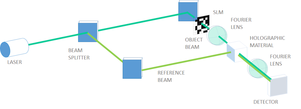
A typical optical layout of page-type holographic data storage (the character code of my name is encoded in binary data in the SLM in this figure).

How to Design a Single-Bit Hologram Simulation

Now, let’s simulate a bit-by-bit holographic data storage example. There is a single open aperture for the object beam instead of an SLM, so the object beam carries one-bit data, which can mean “1 or 0” or “exist or not exist”. Our computational domain is a square and the layout of the beams is such that the object beam enters from the top side, while the reference beam comes from the left. Note that this 90-degree configuration is a simplified example to demonstrate the simulation setup and is not a very realistic scenario.

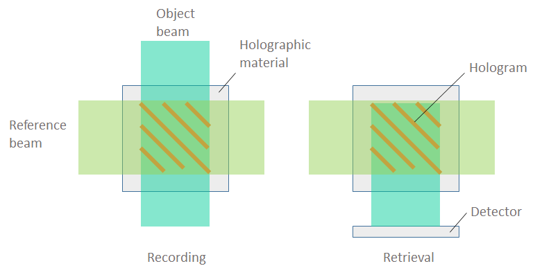
A schematic of bit-by-bit holographic data storage. The objective is to compute the electromagnetic fields within a small region of the holographic material.

Let’s go through each of the steps of the simulation process for holographic data storage, including preparation, recording, retrieval, and an overview of the appropriate settings in COMSOL Multiphysics.

Our first task is to appropriately set up the model of the laser beam. This process looks very simple, but it requires knowledge of electromagnetics and computer simulation beyond just the usage of COMSOL Multiphysics. The following points must be considered when setting up a model of a laser beam.

Beam Collimation

First of all, we want to have straight beams that uniformly propagate through the material and a wide spatial overlap between the two beams. To achieve this, the beam width has to be chosen carefully. The lower bound on the beam width is controlled by the uncertainty principle. If we try to specify a beam width that is very narrow compared to the wavelength, this means that we are trying to specify the position within a very small region. When the position is well specified, the light’s momentum becomes more uncertain, which equivalently leads to more spreading out of the beam and the beam diverges.

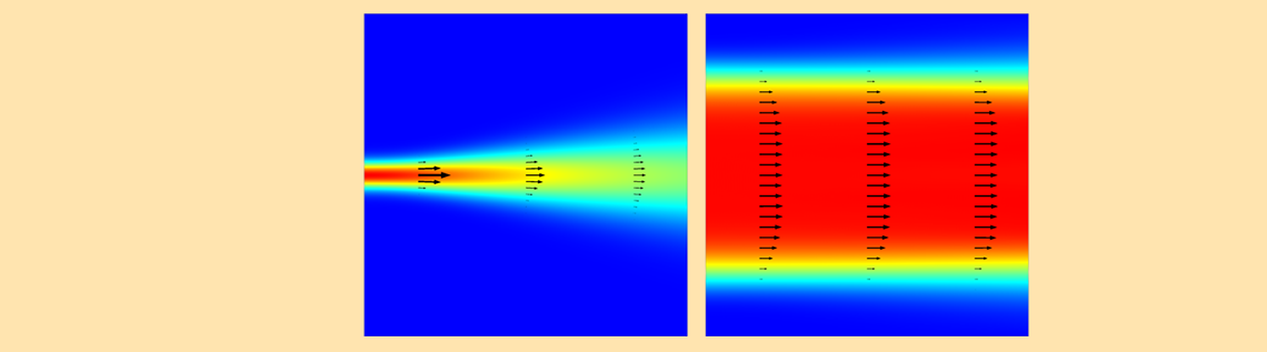
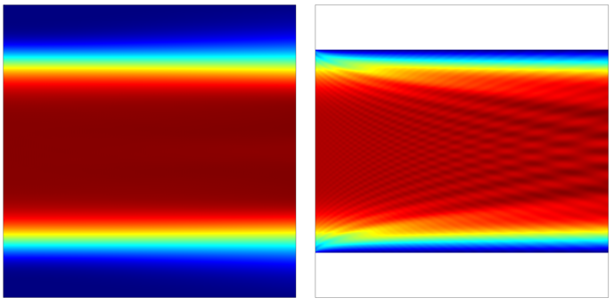
How much the light diverges for a given beam size is quantitatively well described by the paraxial Gaussian beam theory, which defines the beam divergence via the spread angle \theta. This spread angle is related to the paraxial Gaussian beam waist radius w_0 as \tan \theta = \lambda / (\pi w_0), where \lambda is the wavelength. It is obvious from this formula that the light diverges if we make the beam waist radius small compared to the wavelength. In the figure shown below and to the left, we can see a case where the waist radius equals the wavelength. You can see that the small beam waist leads to a quickly diverging beam.

If you instead specify a waist radius ten times the wavelength, then the divergence angle is 1/(10 \pi), which is approximately 32 mrad. This angle is good enough for our purposes. A slightly diverging but almost collimated Gaussian beam is depicted in the figure below on the right. Super Gaussian or Lorentzian beam shapes can also be used to describe such a collimated beam.

A beam with a narrow waist (left) diverges, while a beam with a wide waist (right) diverges negligibly. The electric field magnitude is plotted, along with arrows showing the Poynting vector.

Domain Size

Our modeling domain must be large enough to capture all of the relevant phenomena that we want to capture, but not too large. This can be visualized from the image above of the two crossed beams. The modeling domain need only be large enough to enclose the region where the beams are intersecting. It doesn’t need to be too large, since we aren’t interested in the fields far away from the beam, which we know will be small. The domain also doesn’t need to be too small because we would lose information.

Boundary Conditions

The boundaries of our modeling domain must achieve two purposes. First, we must launch the incoming beams, and second, the beam must be able to propagate freely out of the modeling domain. Within COMSOL Multiphysics, both of these conditions can be realized with the Second-Order Scattering boundary condition, which mimics an open boundary and also allows an incoming field representing a source from outside of the modeling domain to be specified.

It is also important that the scattering boundary conditions are placed far enough away from the beam centerline, such that the beams are only normally incident upon the boundaries. The beam should not have any significant component in parallel incidence upon the boundary, since this will lead to spurious reflections, as described in our earlier blog post on boundary conditions for electromagnetic wave problems.

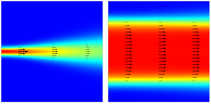
We can use the information about the beam waist to choose a domain size that is sufficiently wider than the beam, such that the electric field intensity falls off by six orders of magnitude at the boundary, as shown in the figure below.

If the domain width relative to the beam width is sufficiently large, there will be no spurious reflections (left). If the scattering boundary conditions are placed too close (right) to the beam centerline, there are observable spurious reflections.

Meshing Requirements

This problem solves for beams propagating in different directions and computes scattering and interference patterns in a material with a known refractive index. Since we know the wavelength and the refractive index, we can use this information to choose the element size. The element size must be small enough to resolve the variations in the propagating electromagnetic waves. We know from the Nyquist criterion that we need at least two sample points per wavelength, but this would give us very low accuracy. A good rule of thumb is to start with an element size of (\lambda/n)/8, or eight elements per wavelength in a material with peak refractive index n.

Of course, you will always want to perform a mesh refinement study. For this type of problem, an element size of (\lambda/n)/16 will typically be sufficient. Also be aware that the smaller you make the elements (the higher the accuracy), the more time and computational resources your model will take. For a detailed discussion about how to predict the size of the model, please see our blog post on the memory needed to solve a model.

Considering all of these factors, we will simulate a laser beam with a vacuum wavelength of 1 um and a beam waist profile of \exp(-y^6/w^6), a sixth-order super Gaussian beam. We will solve for the out-of-plane electric field, which means that we solve a scalar Helmholtz equation.

Simulating the Recording Step

Now that we have appropriate settings for the beam and the domain, we are ready for the recording simulation. The figure below shows the results of the recording process. The object beam and reference beam make an interference fringe pattern at a slant angle of 45 degrees and with a periodicity of 0.524 um. This 45-degree fringe is the cipher for a single of 1 recorded in the holographic material.

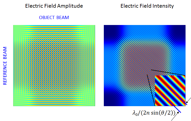
The computed electric field and intensity for the one-bit data recording.

Next, the holographic material modulates its refractive index in the portion where the electric field intensity is above a certain threshold value. In the case of photopolymers, polymerization starts in this high-intensity region. Now, let the distribution of this high-intensity portion be denoted g(x,y), as it adds up modulation on the raw index n_1. This means that the global refractive index n(x,y) can be written as n(x,y) = n_1(x,y) + \Delta n g(x,y). \Delta n is the modulation depth, which is dependent on the material’s photochemical properties.

The function shape of the modulation also depends on the material and process. The new index takes the shape of a biased and periodic rectangular function swinging around the raw index. The next figure plots the new refractive index and its cross section after recording. In this simulation example, we have used n_1=1.35 and \Delta n =0.01. The modulation function g can be expressed by a logical expression, ( (ewfd.normE)/maxop1(ewfd.normE) )>threshold, where the maxop operator calculates the maximum value inside the domain, normalizing the electric field norm. threshold is a given threshold value for polymerization.

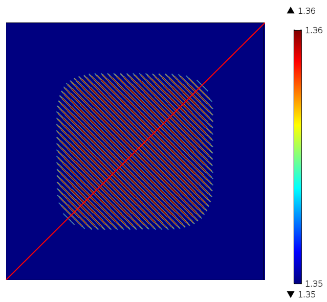
A contour map of the electric field intensity for the binary recording that is cut off at a threshold and binarized.

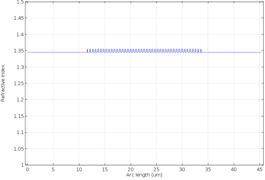
A cross-sectional plot of the modulated index.

Simulating the Retrieval Step

Next, we simulate the retrieval process, which includes:

• Turning off the object beam
• Shining the reference beam only

After these settings change, we get the final results, as shown in the next two plots. The reference beam is diffracted/scattered by the interference fringes and creates a new beam, which restores the amplitude and the phase information overlooking a multiplicative constant. Note that the retrieved object beam is not symmetric because the reference beam slightly diverges.

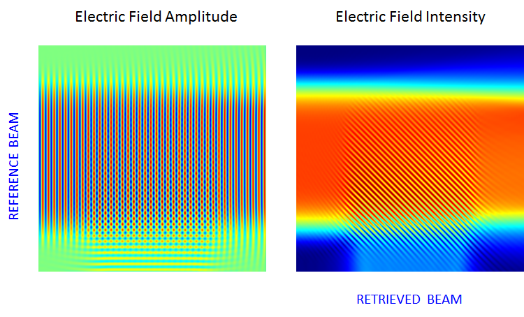
The computed electric field and intensity for the retrieval of the object beam carrying one-bit data.

Automated COMSOL Multiphysics Settings

So far, we have gone through the simulation procedure in a step-by-step manner, but it is possible to perform this sequential simulation all at once. In COMSOL Multiphysics, there is a helpful feature in the Solver settings that we can use to perform this two-step sequence, the recording and retrieval processes, in one click of the Compute button. To do this, we select the Modify physics tree and variables for study step check box in each study step.

For recording, we apply the scattering boundary condition with the incident field of the super Gaussian beam (Reference SBC) on the left edge, the scattering boundary condition with the incident field of the super Gaussian beam (Object SBC) on the top edge, and the scattering boundary condition with no incidence for the rest of the boundaries (Open SBC).

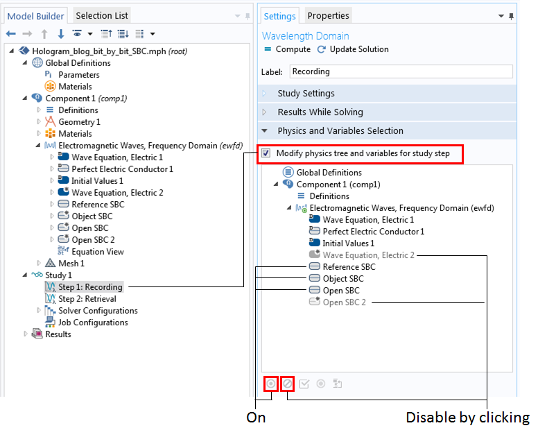
Settings for Study 1 and Step 1 of the recording process.

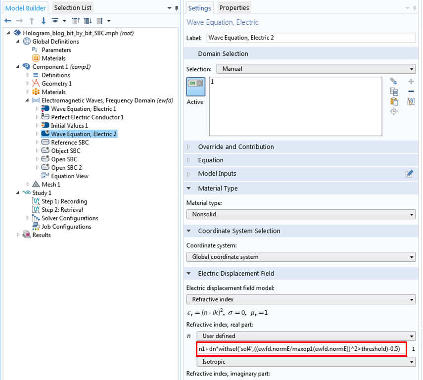
Adding the Wave Equation, Electric 2 node for index modulation.

To set up a modulated refractive index, we add one more Wave Equation, Electric node, in which the previous result specifies a new user-defined refractive index. Here, we have used the withsol() operator, which lets users apply the previous solution to evaluate an arbitrary expression. In this example, the new refractive index is given by n1+dn*withsol('sol2',((ewfd.normE/maxop1(ewfd.normE))^2>threshold)-0.5), where 'sol2' is the solution for Step 1 (the recording process) and the threshold is 0.4.

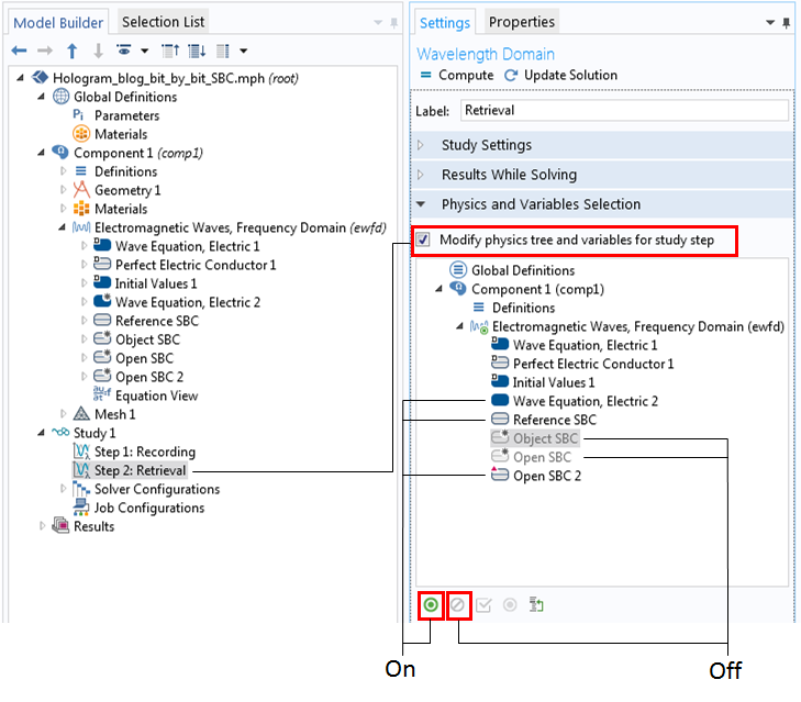
Settings for Study 1 and Step 2 for the retrieval process.

In the retrieval process, we turn off the object beam by disabling the Object SBC. To switch to the modulated refractive index, the original Wave Equation, Electric 1 node is disabled and the Wave Equation, Electric 2 node is turned on. Finally, Open SBC is replaced by a new scattering boundary condition with no incidence for the top, bottom, and right boundaries (Open SBC 2).

Concluding Remarks on Simulating Holographic Data Storage

Today, we discussed how to determine electromagnetic beam settings, which can be a very complex problem. Then, we demonstrated a simple holographic data storage simulation, called a bit-by-bit hologram. We also learned how to implement several steps in COMSOL Multiphysics to run a series of simulation steps at one time. Stay tuned for the next part of this holography series, in which we will simulate a more interesting, complicated, and realistic system of multibit holograms called holographic page data storage.

Further Reading

• Read the blog post Shaping Future Holography for the history, principles, applications, and implications of holograms
• Watch this archived webinar for a full demonstration on how to simulate wave optics problems in COMSOL Multiphysics
• Have any questions? Contact us for support and guidance on modeling your own holography problems in COMSOL Multiphysics