
Until the early 1900s, shock waves were an academic problem studied from a theoretical point of view only. Many great scientists, including Lord Rayleigh, worked on the field until the theory of inviscid shock waves was established in the 1920s. During World War II, this theory started to be applied, mostly to supersonic vehicles. To study shock waves, one important gas dynamic instrument is the shock tube, which is used to test supersonic and hypersonic flows and high-temperature gases.
Shock Waves: Faster than the Speed of Sound
A shock wave is a propagating discontinuity in a flow that travels faster than the speed of sound. Shocks are very thin, leading to very large gradients of velocity and temperature. Hence, shock waves are dissipative, irreversible processes that generate entropy and compress the flow. Static pressure, density, and temperature are increased after the shock.
Shock waves are generated in a number of ways, creating violent changes in pressure. Take thunder, for example: The sudden heating caused by lightning makes the air around it expand faster than the speed of sound, which changes the air pressure and thus creates shock waves. These waves reach our ears a few seconds later as rumbling thunder. The rumbling sound occurs because a lightning bolt is a series of short bursts chained together and the resulting shock waves, which are generated at different altitudes, reach your ears at different times. You might also associate these powerful shock wave blasts with explosions or supersonic flight.

Lightning rapidly heats the air, leading to powerful shock waves that we hear as thunder. Image by Hansueli Krapf — Own work. Licensed under CC BY-SA 3.0, via Wikimedia Commons.
Shock waves have unique properties that set them apart from sound waves. They travel faster than the speed of sound and also decrease in intensity faster than a sound wave. These properties must be accounted for when designing applications such as transonic diffusers, which use shocks to slow down airflow. However, studying shock waves can be challenging due to the abrupt way they are generated. That’s where shock tube experiments come in.
Using Shock Tubes to Better Understand Shock Waves
Shock tubes are instruments used in the testing of supersonic bodies as well as the study of compressible flow phenomena, high-temperature gases, and gas-phase combustion reactions. They consist of a tube closed at both ends and a diaphragm blocking any flow within the tube. The experiments can be conducted in the following steps:
- Increasing the pressure on one side of the tube by using a compressor
- Breaking the diaphragm to start the flow
- Observing the gas through which shock waves propagate as they expand down the other side of the tube
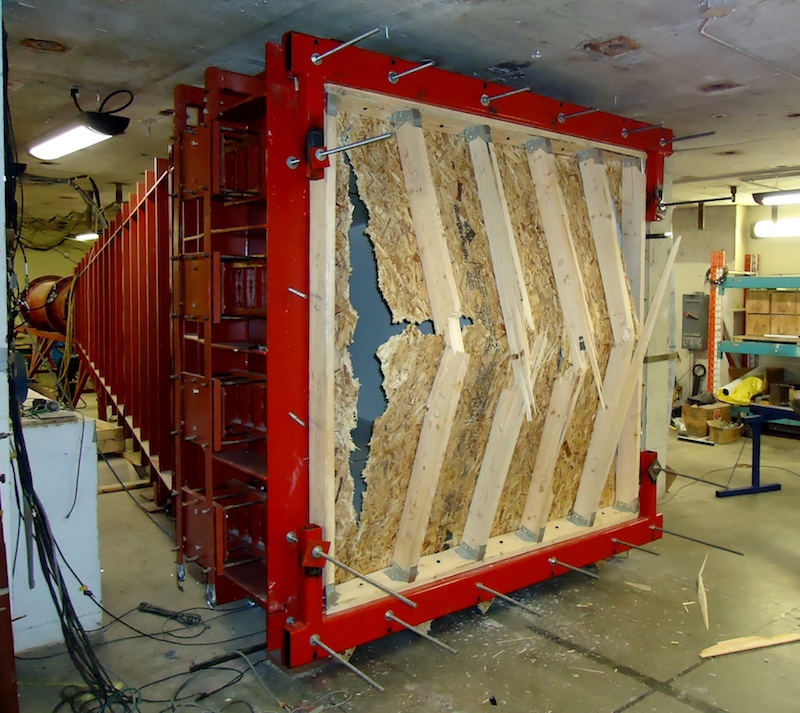
A shock tube test apparatus at the University of Ottawa, Canada. Image by Christian Viau — Own work. Licensed under CC BY-SA 4.0, via Wikimedia Commons.
Shock waves are not the only propagating disturbances observed in shock tube experiments. Expansion fans travel in the opposite direction of shock waves and tend to expand the flow smoothly and continuously. The values of static pressure, density, and temperature are decreased across the expansion fan, and entropy is conserved; this process is hence reversible. Another disturbance observed in shock tubes is contact waves or contact surfaces. Contact surfaces are the interface across which gases mix and separate. Note that contact waves propagate discontinuities in the density, but velocity and pressure are constant across them.
Instead of setting up a physical shock wave experiment, you can save time and resources by studying shock waves via a simulation application created using the Application Builder in the COMSOL Multiphysics® software. As an example, let’s examine a shock tube simulation application that solves for the density, momentum, and internal energy inside the contained tube.
Calculating the Flow in a Shock Tube with a Numerical Modeling Application
The flow in shock tubes is convection-dominated and reaches high Mach numbers. The effects of heat conduction and viscosity are rather small and can be neglected. Inviscid compressible flows can thus be modeled using the Euler equations of gas dynamics.
The shock tube application makes use of the Wave Form PDE interface to solve the 1D compressible Euler equations in time and space using explicit Runge-Kutta time stepping in combination with a piecewise constant discontinuous Galerkin method in space. The dependent variables are the density, momentum, and internal energy. Other variables, such as pressure, velocity, and temperature, can be obtained as a combination of the dependent variables. Using the shock tube application, you can solve for a wide range of combinations of initial conditions.
An application such as this one provides a dedicated interface that allows you to run complex simulations without having to dive into the technicalities of mathematical modeling, and without having to know how to set up a model in COMSOL Multiphysics. Simulation applications can be deployed to others with COMSOL Server™ or COMSOL Compiler™ so that specialists, design teams, and R&D teams can run their own analyses.
For more details on the design of the shock tube simulation application, see the documentation here.
Evaluating the Simulation Results
A common test used to check the accuracy of computational fluid codes dealing with compressible flow is Sod’s shock tube problem (Ref. 1). We use the shock tube application to solve the shock wave proposed by Sod in a 20-m-long shock tube. A diaphragm in the middle separates two regions of air at different values of pressure and density: 105 Pa and 1 kg/m3 to the left and 104 Pa and 0.125 kg/m3 to the right.
The results below show the density, pressure, and velocity distributions within the tube, with the y-axis representing time and the x-axis displaying the position across the tube with respect to the diaphragm. The three plots show the presence of a shock traveling to the right and an expansion fan propagating to the left. A contact wave is observed as a discontinuity in the density that moves to the right slower than the shock wave. The shock wave is reflected once it reaches the wall of the tube and interacts with the contact wave.


The density (left), pressure (middle), and velocity (right) distributions in Sod’s shock tube problem.
As the results show, you can accurately study shock waves in a shock tube by building a simulation application like the one discussed here.
Next Steps
To get inspiration for building your own simulation applications, try the shock tube application by clicking the button below. You’ll be taken to the Application Gallery, where you can download the documentation and MPH file by logging into your COMSOL Access account.
Learn more about shock wave simulation by reading this blog post on how to model supersonic flows.
Reference
- G.A. Sod, “A Survey of Several Finite Difference Methods for Systems of Nonlinear Hyperbolic Conservation Laws,” J. Computational Physics, vol. 27, pp. 1–31, 1978.


Comments (0)