

Zone electrophoresis separates different species in a sample into distinct well-resolved peaks, giving scientists the ability to analyze substances like proteins and nucleic acids. Improving this electrophoretic separation technique requires us to accurately model the transport and separation of these species. Here, let’s look at how the COMSOL Multiphysics® software can be used to simulate the movement of species during zone electrophoresis.
What Is Zone Electrophoresis?
Zone electrophoresis is a process in which a sample containing different species is transported through a continuous electrolyte buffer system exposed to a potential gradient. The different species have different mobilities, which causes them to eventually form separate well-resolved peaks.
Using zone electrophoresis, scientists can study nucleic acids, biopolymers, proteins, and more. Thus, this technique has a variety of potential applications. For instance, one type of zone electrophoresis (capillary zone electrophoresis) is used in the field of forensic science.
Simple schematic depicting capillary zone electrophoresis. Original image by Ccl005, “CZE” — Own work. Licensed under CC BY-SA 3.0, via Wikimedia Commons.
When studying zone electrophoresis, it’s important to accurately model the transport and concentration of different species. To do so in an efficient manner, we can turn to COMSOL Multiphysics and the Electrophoretic Transport interface.
Modeling Zone Electrophoresis with COMSOL Multiphysics®
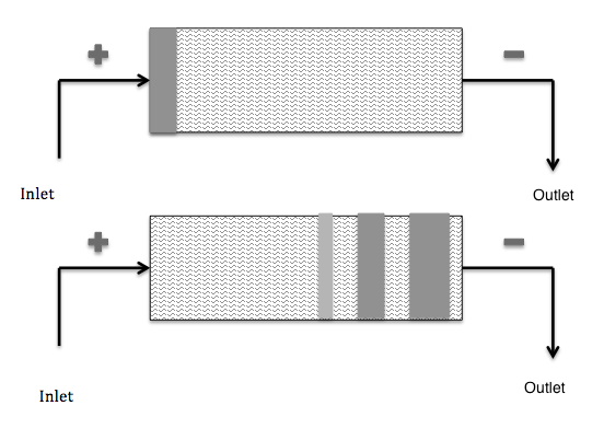
The geometry of our model consists of a 20-cm separation column (represented by a line in 1D), with a current density of 2500 A/m2 applied to the end of the column. The domain boundaries face reservoirs full of the buffer electrolyte needed for the zone electrophoresis process.
In the model, we account for the transport of four different species: acetic acid and tris(hydroxymethyl)aminomethane (“tris”) as the buffer solution, and aniline and pyridine as the sample that we are trying to separate. For each of these species, we specify mobility, acid constant, initial conditions, and boundary conditions. Also, the self-ionization of water is included as an equilibrium reaction in the model.
To better study the transport of the acid and bases in our model, we use the Electrophoretic Transport interface, new in version 5.3 of COMSOL Multiphysics. This interface is made for modeling electrophoresis modes, such as zone electrophoresis, isoelectric focusing, and moving-boundary electrophoresis. The interface also helps solve for the species concentration, pH, and electrolyte potential distributions — the results of which we discuss in the next section.
Zone electrophoresis separating pyridine and aniline into distinct peaks.
Evaluating the Simulation Results
We use a time-dependent solver to study the zone electrophoresis process over a 5-minute time period. The pH distribution and electrolyte conductivity both have a rectangular imprint at the initial sample concentration (0 minutes). After 4 minutes have passed, these distribution patterns become more complex.


Comparison of the pH distribution (left) and electrolyte conductivity (right) at 0 and 4 minutes.
Next, let’s check how the concentration distribution of the buffer electrolyte species, tris and acetic acid, change over time. The results below indicate that after 4 minutes, the initial position of the sample appears as “ghost” peaks within the buffer electrolyte.


Comparison of the tris (left) and acetic acid (right) concentration distributions at 0 and 4 minutes.
For the other two species of interest, pyridine and aniline, we compare their concentrations at 1 and 3 minutes. These plots show that as time passes and the samples move to the right of the separation column, the distance between the triangular peaks increases.
These results indicate that in the simulation, zone electrophoresis successfully separates a mixed sample of pyridine and aniline into two well-resolved concentration peaks.


Comparison of the concentration distribution of pyridine and acetic acid at 1 (left) and 3 (right) minutes.
Of course, this simple example is only the start of what you can do with the Electrophoretic Transport interface. Give the model a try by downloading the tutorial below.

Comments (0)