
Using Perfectly Matched Layers and Scattering Boundary Conditions for Wave Electromagnetics Problems
When solving wave electromagnetics problems, it is likely that you will want to model a domain with open boundaries — that is, a boundary of the computational domain through which an electromagnetic wave will pass without any reflection. COMSOL Multiphysics offers several solutions for this. Today, we will look at using scattering boundary conditions and perfectly matched layers for truncating domains and discuss their relative merits.
Why Truncate the Domain?
We are often interested in modeling a radiating object, such as an antenna, in free space. We may be building this model to simulate an antenna on a satellite in deep space or, more often, an antenna mounted in an anechoic test chamber.
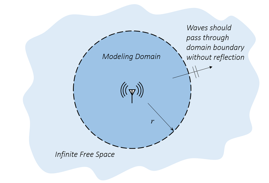
An antenna in infinite free space. We only want to model a small region around the antenna.
Such models can be built using the Electromagnetic Waves, Frequency Domain formulation in the RF Module or the Wave Optics Module. These modules provide similar interfaces for solving the frequency domain form of Maxwell’s equations via the finite element method. (For a description of the key differences between these modules, please see my previous blog post, titled “Computational Electromagnetics Modeling, Which Module to Use?“)
Let’s limit ourselves in this blog post to considering only 2D problems, where the electromagnetic wave is propagating in the x-y plane, with the electric field polarized in the z-direction. We will additionally assume that our modeling domain is purely vacuum, so that the frequency domain Maxwell’s equations reduce to:
where E_z is the electric field, relative permeability and permittivity \mu_r = \epsilon_r = 1 in vacuum, and k_0 is the wavenumber.
Solving the above equation via the finite element method requires that we have a finite-sized modeling domain, as well as a set of boundary conditions. We want to use boundary conditions along the outside that are transparent to any radiation. Doing so will let our truncated domain be a reasonable approximation of free space. We also want this truncated domain to be as small as possible, since keeping our model size down reduces our computational costs.
Let’s now look at two of the options available within the COMSOL Multiphysics simulation environment for truncating your modeling domain: the scattering boundary condition and the perfectly matched layer.
The Scattering Boundary Condition
One of the first transparent boundary conditions formulated for wave-type problems was the Sommerfeld radiation condition, which, for 2D fields, can be written as:
where r is the radial axis.
This condition is exactly non-reflecting when the boundaries of our modeling domain are infinitely far away from our source, but of course an infinitely large modeling domain is impossible. So, although we cannot apply the Sommerfeld condition exactly, we can apply a reasonable approximation of it.
Let’s now consider the boundary condition:
You can clearly see the similarities between this condition and the Sommerfeld condition. This boundary condition is more formally called the first-order scattering boundary condition (SBC) and is trivial to implement within COMSOL Multiphysics. In fact, it is nothing other than a Robin boundary condition with a complex-valued coefficient.
If you would like to see an example of a 2D wave equation implemented from scratch along with this boundary condition, please see the example model of diffraction patterns.
Now, there is a significant limitation to this condition. It is only non-reflecting if the incident radiation is exactly normally incident to the boundary. Any wave incident upon the SBC at a non-normal incidence will be partially reflected. The reflection coefficient for a plane wave incident upon a first-order SBC at varying incidence is plotted below.
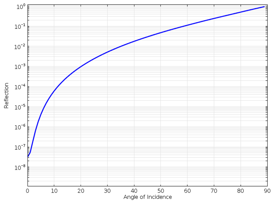
Reflection of a plane wave at the first-order SBC with respect to angle of incidence.
We can observe from the above graph that as the incoming plane wave approaches grazing incidence, the wave is almost completely reflected. At a 60° incident angle, the reflection is around 10%, so we would clearly like to have a better boundary condition.
COMSOL Multiphysics also includes (as of version 4.4) the second-order SBC:
This equation adds a second term, which takes the second tangential derivative of the electric field along the boundary. This is also quite easy to implement within the COMSOL software architecture.
Let’s compare the reflection coefficient of the first- and second-order SBC:
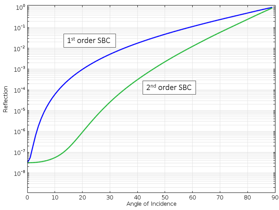
Reflection of a plane wave at the first- and second-order SBC with respect to angle of incidence.
We can see that the second-order SBC is uniformly better. We can now get to a ~75° incident angle before the reflection is 10%. This is better, but still not the best we can achieve. Let’s now turn our attention away from boundary conditions and look at perfectly matched layers.
The Perfectly Matched Layer
Recall that we are trying to simulate a situation such as an antenna in an anechoic test chamber, a room with pyramidal wedges of radiation absorbing material on the walls that will minimize any reflected signal. This can be our physical analogy for the perfectly matched layer (PML), which is not a boundary condition, but rather a domain that we add along the exterior of the model that should absorb all outgoing waves.
Mathematically speaking, the PML is simply a domain that has an anisotropic and complex-valued permittivity and permeability. For a sample of a complete derivation of these tensors, please see Theory and Computation of Electromagnetic Fields. Although PMLs are theoretically non-reflecting, they do exhibit some reflection due to the numerical discretization: the mesh. To minimize this reflection, we want to use a mesh in the PML that aligns with the anisotropy in the material properties. The appropriate PML meshes are shown below, for 2D circular and 3D spherical domains. Cartesian and spherical PMLs and their appropriate usage are also discussed within the product documentation.
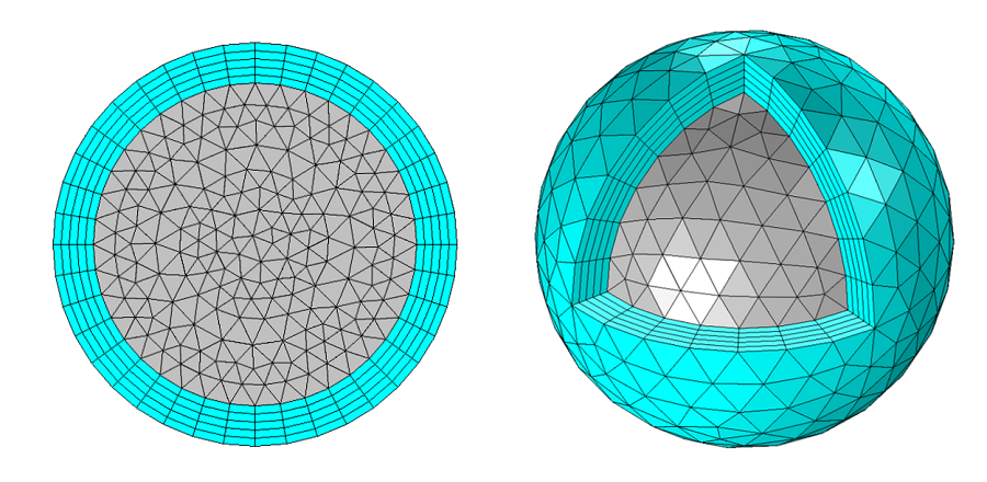
Appropriate meshes for 2D and 3D spherical PMLs.
In COMSOL Multiphysics 5.0, these meshes can be automatically set up for 3D problems using the Physics-Controlled Meshing, as demonstrated in this video.
Let’s now look at the reflection from a PML with respect to incident angle as compared to the SBCs:
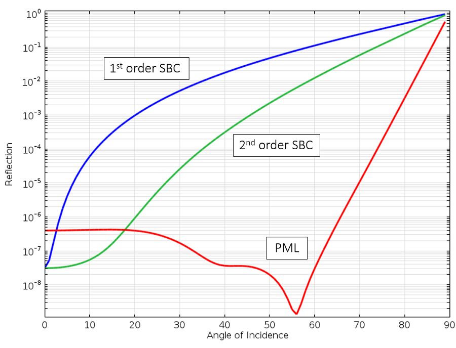
Reflection of a plane wave at the first- and second-order SBC and the PML with respect to angle of incidence.
We can see that the PML reflects the least amount across the widest range. There is still reflection as the wave is propagating almost exactly parallel to the boundary, but such cases are luckily rather rare in practice. An additional feature of the PML, which we will not go into detail about for now, is that it absorbs not only the propagating wave, but also any evanescent field. So, from a physical point of view, the PML truly can be thought of as a material with almost perfect absorption.
So Which Option Should You Use?
Clearly, the PML is the best of the approaches described here. However, the PML does use more memory as compared to the SBC.
So, if you are early in the modeling process and want to build a model that is a bit less computationally intensive, the second-order SBC is a good option. You can also use it in situations where you have a strong reason to believe that any reflections at the SBC won’t greatly affect the results you are interested in.
The first-order SBC is currently the default, for reasons of compatibility with previous versions of the software, but with COMSOL Multiphysics version 4.4 or greater, use the second-order SBC. We have only introduced the plane-wave form of the SBC here, but cylindrical-wave and spherical-wave (in 3D) forms of the first- and second-order SBC’s are also available. Although they do use less memory, they all exhibit more reflection as compared to the PML.
The SBC and the PMLs are appropriate conditions for open boundaries where you do not know much about the fields at the boundaries a priori. If, on the other hand, you want to model an open boundary where the fields are known to have a certain form, such as a boundary representing a waveguide, the Port and Lumped Port boundary conditions are more appropriate. We will discuss those conditions in an upcoming blog post.


Comments (12)
Mahendar Kumbham
January 29, 2015Thank you very much for simple and effective info. We hope many like this from you in future. Although I am working from 1 year on EM wave, I never realized that second order SBC is there in 4.4 version. Thank you so much.
Ravinder
January 30, 2015Thank you very much for updating us. this information is very useful for simulating em wave propagation with open boundaries.
Please keep updating on this.
Krupali
February 1, 2015This article is very helpful to comsol users to understand exact difference b/w these two BC.It solve my doubt regarding 1st and 2nd order SBC.Thank you so much for nicely representation.
Keep updating!
Alejandro Cebrecos Ruiz
April 22, 2015Thanks so much for this brief and really clear and practival explanation on Radiation Conditions and PML. I found them very useful
Katerina
April 7, 2016Thank you for the explanation. It was very clear.
Chirag M Patil
November 9, 2016Thank you for the clear insights into SBC and PML. How far should the SBC be defined from the active domain, for it to behave as a nonreflecting boundary condition?
Nathan Woodard
February 23, 2017Nice write up. Much appreciated!
Felipe Marcolino
April 20, 2017Thank you for the clarifications.
Mohammad Saiful Islam
January 15, 2019Excellent clarifications on the boundary conditions. It is very clear and helpful.
昊 吴
October 18, 2021Thank you very much for this blog. Very clear!
Chris Scheffler
March 23, 2022Hello, I am interested in reprinting a figure from this post in an academic thesis. I’m wondering who I need to contact to request permission? Thank you for your time.
Sarra Chabbar
May 9, 2023Thank you very much for the explanation.