The algebraic multigrid (AMG) solver provides robust solutions for large CFD simulations. Available as of version 5.3a of the COMSOL Multiphysics® software, the AMG method only requires one mesh, in contrast to the geometric multigrid (GMG) solver, which requires at least one extra coarser mesh. This eliminates the hassle associated with creating coarse meshes for complex geometries with small details that are difficult to mesh unless a fine mesh is used.
A Fluid Flow Problem, Mathematical Model, and Numerical Model
Fluid flow can be accurately described by the laws for conservation of momentum, mass, and energy. The most accurate way to describe these laws is by partial differential equations (PDEs). The system of PDEs that describes these laws is nonlinear. In most practical cases, these equations cannot be solved analytically. Instead, we can discretize in space and time in order to get an approximation of the PDEs in the form of algebraic equations that we can solve. We can say that we approximate our mathematical model with a numerical model.
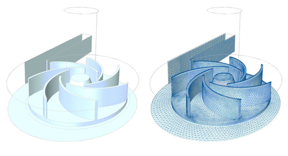
The “real” description of the geometry, to the left, is approximated with a discretized description where momentum balances and mass balances in each element are carried out.
For problems in space and time, COMSOL Multiphysics uses the method of lines, where the discretization in space is done using the finite element method and time discretization is done using some standard method for ordinary differential equations, such as backwards differentiation formula (BDF) or Generalized-α.
The fluid flow equations are nonlinear, which means that the discretized numerical model equations are also nonlinear. For transient problems, a system of nonlinear equations has to be solved at every time step. For steady flows, the numerical model equations form a system of nonlinear equations that has to be solved once.
The method for solving the systems of nonlinear equations, both for the time-dependent and stationary problems, is a damped Newton method, when the system is solved fully coupled. This method is based on linearization of the nonlinear equations and solving the linear equations in a sequence of iterations, often referred to as Newton iterations, until we obtain the desired accuracy.
Why Should I Use Iterative Methods for Linear Equation Systems?
In our case, we have hundreds of thousands or millions of equations and unknowns, proportional to the number of nodes in the finite element mesh that we used to generate the numerical equations. The linear equation system that has to be solved in each Newton iteration is too expensive to solve with a direct solver. However, we can solve the linear equations with an iterative solver using much less memory.
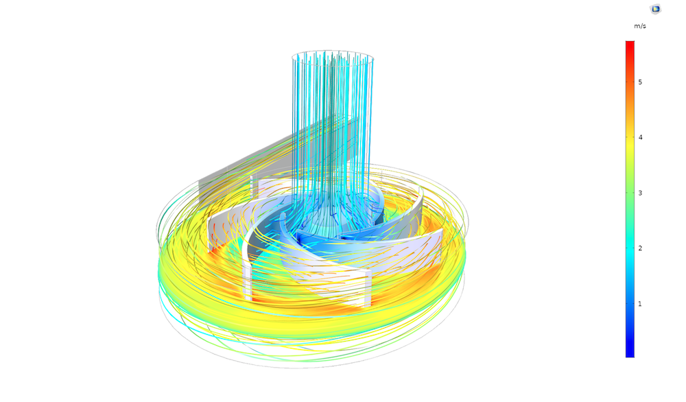
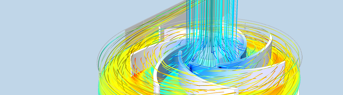
Even this relatively simple model of the flow in a centrifugal pump requires 350,000 equations and unknowns. Thanks to the AMG solver, the equations can be solved on a desktop computer.
For fluid flow problems, COMSOL Multiphysics uses the generalized minimal residual (GMRES) method, which is an iterative method for solving very large systems of linear equations. We can modify the linear equation system so that the GMRES method performs much better.
Multigrid Methods
Multigrid methods provide an optimal technology for modifying, or preconditioning, the equation system for iterative techniques like the GMRES method.
The GMG method acts on the linear equation system for different mesh levels, from fine to coarse meshes. It transfers solution candidates, the iterates, between different linear systems corresponding to coarser and finer meshes. The idea is that a direct method is solved only for the coarsest mesh and this information is used to find a solution for the finer mesh levels more quickly. The coarse problem needs to be so small that it does not affect the performance of the method.
In each GMRES iteration, the GMG method may go from a finer mesh, where the right-hand side of the system is obtained, mapping the approximate solutions at the finer levels to the coarser mesh in a process called presmoothing. The solution of the equations is corrected at the coarsest level using a direct solver. This solution is then mapped to the fine levels again, in a process called postsmoothing.
The process of going down and up the mesh levels (V-cycle) can be repeated for each GMRES iteration. When the tolerance in the GMRES iterations is reached, we have a good-enough solution to the linear system.
Why Should I Use the AMG Method?
The GMG method is extremely efficient for fluid flow problems. However, it has a very serious limitation. For complex geometries, it may be difficult or almost impossible to generate a coarse mesh that gives a system of equations that is small enough to be solved at the coarsest level.
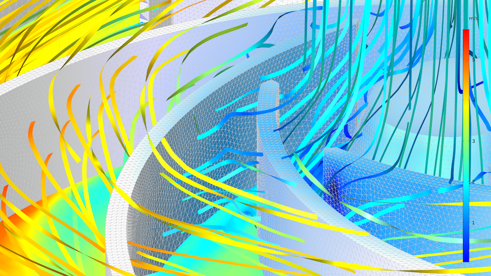
The thin blades of the centrifugal pump result in very small elements in the fluid around the blades. This also implies that even the coarsest mesh level generates too many elements and consequently too many equations to be solved with a direct solver using GMG.
The AMG method does not require different mesh levels. The coarsening process in the AMG method is based only on the structure of the linear system of equations, or, more precisely, on the matrix that represents the left-hand side of the equation system. The method agglomerates entries in the matrix that are connected into fewer entries into a new matrix with smaller size. The process of agglomerating entries can be repeated and even smaller matrices can be constructed. These are then assigned different levels according to how many aggregations have been performed. The principle of the multigrid cycle with presmoothing, postsmoothing, and coarsest level solve is then the same as for the GMG method for the constructed matrices at the different levels.

The settings for the iterative solver (GMRES) used in combination with the AMG method to solve the model equations for the Ahmed body shown below. Note that the method is used to solve for the momentum and continuity equations (u, v, w, p) and for the turbulence model variables (k, ε) in two separate steps in the segregated solver.
What About Performance?
In order to monitor the performance of the different solver settings in COMSOL Multiphysics, a couple thousand tests are run every day. One of the test cases for iterative solvers and fluid flow is the so-called Ahmed body model. Another test is the so-called laminar static mixer test. The results of the measurements show that for 6.3 million degrees of freedom, the AMG method beats the GMG method with about a 13% shorter solution time on a single-core computer.
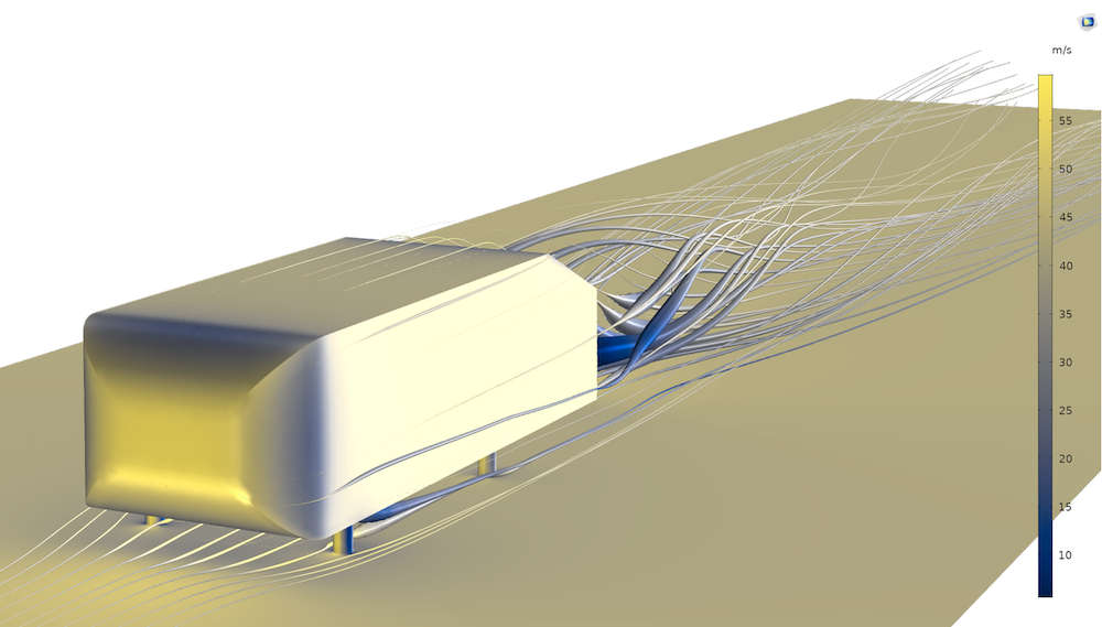
The Ahmed body is a benchmark model for turbulent flow and a verification model for turbulence models in general.
Note that these results reflect the COMSOL Multiphysics implementation of these methods, not a general property of the methods. On a computer with four cores, this difference drops to around 6%. For 32 cores, the two methods are equal. The reason for this behavior is that the GMG solver is parallelized to a higher degree than the AMG solver. The new AMG method has already in its first year shown superior robustness and excellent performance, on par with the best-case scenario for the GMG method.
Next Steps
Learn more about the key features of COMSOL Multiphysics for your numerical modeling needs via the button below.
Read more about using multigrid methods on the COMSOL Blog:


Comments (5)
Trevor Munroe
March 27, 2018Is the pump model available, Ed?
Ed Fontes
April 5, 2018 COMSOL EmployeeHi Trevor.
The pump is not available yet but it will be available in the product update soon. Meanwhile, there is a smaller but similar problem:
https://www.comsol.com/model/centrifugal-pump-44191
Best regards,
Ed
Ed Fontes
April 5, 2018 COMSOL EmployeeThe updated model used in the blog post is now available in the same entry as above:
https://www.comsol.com/model/centrifugal-pump-44191
Best regards,
Ed
Michael Rembe
November 30, 2018Hi Ed,
in my 3D cavern flow model I use P2-P2 elements. These are necessary or advantageous because of the strong buoyancy force. What do you think about this solver setting:
GMRES -> GMG as preconditioner only to reduce the higher order; coarse solver SAMG. It runs and the GMG doesn’t need a coarse mesh. The benchmark shows that GMG with SAMG as coarse solve is faster than SAMG with Pardiso as coarse solver.
Best regards
Michael Rembe
Ed Fontes
November 30, 2018 COMSOL EmployeeHi Michael,
It sounds like a very good approach! Using higher order elements gives you an extra mesh level with the same mesh, so it is a smart approach for GMG-SAMG. We are actually using the same approach in LES simulations with p2-p2 elements.
We do not have a way of reducing the order with SAMG yet, but we are working on it. Then this will be identical to what you are doing.
Best regards,
Ed