

The battery modeling interfaces in COMSOL Multiphysics use predefined equation sets based on established modeling frameworks. However, the software is not limited to these predefined formulations: Equation-based interfaces can be used to introduce custom equations, along with access to the equations implemented in the built-in physics interfaces. This blog post will cover the flexibility and customization capabilities of COMSOL Multiphysics for battery modeling.
Why Customization May Be Needed
Established modeling frameworks, such as the Doyle–Fuller–Newman (DFN) model, the single-particle model (SPM), the single-particle model with electrolyte (SPMe), and the lumped battery models, are commonly used to study battery performance under a range of operating conditions. As advances in electrode materials, cell chemistries, and cell designs continue to introduce new physical effects and behaviors, extending the underlying battery model to account for phenomena specific to particular materials and chemistries may sometimes be necessary to accurately capture overall cell behavior. With COMSOL Multiphysics, users can modify or extend existing formulations and investigate proposed model developments.
Battery Model Workflow
The general workflow for setting up battery models in COMSOL Multiphysics is straightforward. The governing equations that describe the cell’s electrochemical behavior are predefined and embedded in the battery interfaces. To define the battery cell of interest, the user specifies its geometry, materials, operating conditions, and other required inputs and parameters.
Each battery interface clearly identifies its underlying modeling framework and provides easy access to the corresponding governing equations. Rather than functioning as a black box in which internal workings are hidden, the interface exposes its underlying formulations, enabling users to modify existing equations or introduce new ones as needed.
This flexibility is becoming increasingly important as battery research continues to advance. New electrode materials are being explored for both established technologies, such as lithium-ion batteries, and emerging battery chemistries. Each material can introduce distinct behavior that may need to be represented in the model. Examples include voltage hysteresis, electrochemical-mechanical effects caused by material expansion and contraction, and particle-size heterogeneity in battery electrodes. Extending or modifying existing battery modeling frameworks allows these new materials, mechanisms, and physical effects to be incorporated without requiring users to build the entire model from scratch.
Understanding the Framework Before Customization
Before extending or customizing a model, it is helpful to understand the underlying modeling framework. This includes knowing which equations are solved, the physical phenomena they represent, how the dependent variables are coupled, and how the equations work together. Familiarity with the physics interface is also useful, particularly the nodes in the Model Builder associated with each part of the formulation and the locations of relevant inputs, variables, and equations. The COMSOL documentation supports this process by providing the governing theory, mathematical formulations, and information about each built-in feature.
Three Levels of Model Customization
Once the framework is understood, the next step is to define the objective of the customization. Model customization can generally be implemented at three levels.
At the first level, model inputs such as kinetic, thermodynamic, and transport properties can be modified. User-defined options in the corresponding menus make it possible to enter custom expressions for material properties and reaction kinetics.
At the second level, users can introduce additional equations. COMSOL provides several equation-based modeling interfaces for defining partial differential equations (PDEs), ordinary differential equations (ODEs), differential–algebraic equations (DAEs), and algebraic equations, either globally or distributed over spatial domains. Variables solved for using these interfaces can be coupled seamlessly with variables from the built-in physics interfaces and used as inputs to those interfaces. You can learn more about equation-based modeling in COMSOL Multiphysics here.
At the deepest level, users can modify or replace parts of the built-in domain or boundary equations in the physics interfaces. This type of low-level customization generally requires familiarity with the weak-form formulation (more information).
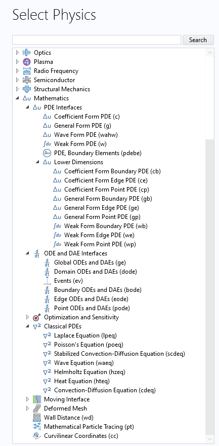
The equation-based interfaces can be accessed and added to a model by expanding the Mathematics branch in the Select Physics window.
Particle Transport Equation in the DFN Model
Now, let’s consider an example. In the DFN framework, solid-state lithium transport within active material particles is commonly described by a Fickian diffusion equation. In the Lithium-Ion Battery interface, this formulation is available as a built-in particle transport model. In the Model Builder tree, when a Porous Electrode node is configured with intercalating particles, the Particle Intercalation subnode defines the particle-scale transport formulation. COMSOL then introduces an additional particle coordinate as an extra abstract dimension and solves the governing equation together with its boundary conditions.
The particle model requires inputs such as the intercalation diffusivity, particle radius and type, and active material volume fraction. Once these inputs are defined, the particle transport equation is solved for the solid-phase lithium concentration. At the particle center, a zero flux boundary condition is imposed due to symmetry. At the particle surface, the lithium flux is determined by the reaction current density calculated using the electrode kinetics formulation specified in the Porous Electrode Reaction subnode.
For the transport model, as shown in the screenshot below, the interface offers users three menu options to choose from: Fick’s law, which is the default; the Baker–Verbrugge formulation, which introduces a correction to the diffusion coefficient based on the equilibrium potential of the intercalation reaction; and No spatial gradients, which reduces the equation in the extra dimension to an ODE, as explained in the following section.
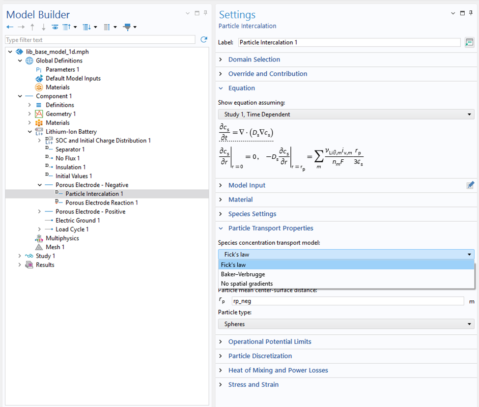 Settings window for the Particle Intercalation node showing the available transport models: Fick’s law, Baker–Verbrugge, and No spatial gradients.
Simplifying Particle Transport to an ODE
When the No spatial gradients option is selected, particle transport is simplified by assuming that the concentration is uniform within each particle. The spatially resolved Fickian diffusion PDE is therefore replaced by an ODE for the average particle concentration. As mentioned earlier, the local charge transfer current density calculated in the Porous Electrode Reaction node serves as the source term for this ODE. This current density can be customized by selecting User defined for the electrode kinetics and specifying a custom charge transfer expression. This makes it possible to include additional contributions to the local current density and, consequently, to the source term in the particle concentration balance.
The Application Library contains two tutorial models that demonstrate hysteretic behavior in active electrode materials: one for lithium iron phosphate (LFP) and one for silicon. Both materials have attracted considerable interest for use in lithium-ion batteries. In each model, particle transport is represented using the No spatial gradients option. The models also show how equation-based interfaces can be coupled with the Lithium-Ion Battery interface to introduce additional variables and equations.
In the silicon example, the built-in Lithium insertion kinetics are used without modification, while an additional memory variable is defined over the blended electrode domain using an equation-based interface. This memory variable models voltage hysteresis by controlling the transition between the lithiation and delithiation equilibrium potentials. In the LFP example, separate concentration variables are introduced for the lithium-poor and lithium-rich phases, each governed by a Domain ODEs and DAEs interface (more information), making both concentrations spatially defined throughout the porous electrode. For each phase, separate expressions for the equilibrium potential, exchange current densities, and local current densities are used to calculate the corresponding contribution to the local current density. The average particle concentration is solved for by the Lithium-Ion Battery interface, with its source term defined as the total local current density, obtained by weighting the contributions from the lithium-poor and lithium-rich phases by their respective volume fractions. Together, these phase-specific formulations provide a simplified approach for capturing voltage hysteresis in a porous LFP electrode.
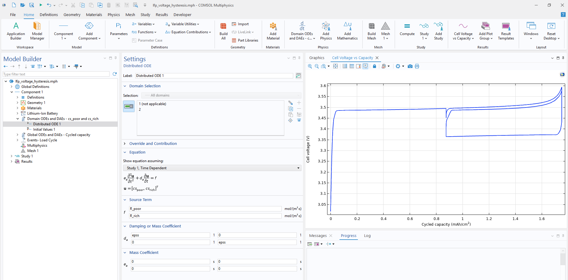 Implementation of the lithium-poor and lithium-rich phase concentrations using a Domain ODEs and DAEs interface, where the equations are defined by specifying the source terms and relevant coefficients, shown alongside the resulting cell voltage.
These examples demonstrate two proposed approaches for modeling voltage hysteresis. Because additional models of voltage hysteresis and particle transport in these materials are still being investigated by the battery research community, users may wish to implement alternative or more advanced formulations. Depending on the formulation, this may involve adding contributions to the built-in Fickian particle transport equation or replacing it entirely. The following section describes how to disable the built-in particle transport formulation so that the governing domain and boundary equations can be defined manually.
Extending Particle Transport at the Lowest Level
When spatial concentration gradients within the particles must be retained, and more control over the particle transport equation is needed, users can manually define the governing equation in the extra dimension.
As noted earlier, this approach requires some familiarity with weak-form formulations, but it enables battery modelers to incorporate additional physics or modify existing formulations within the DFN model. AI-assisted tools can help lower the barrier by explaining weak-form expressions, suggesting initial formulations, or helping translate governing equations into a form suitable for implementation.
The first step to manually define the equation is to click the Show More Options button, represented by an eye icon in the Model Builder toolbar, and enable the Extra Dimensions and Equation Contributions checkboxes in the dialog, as illustrated in the screenshot below. Enabling these options allows extra dimension components to be added under Global Definitions and provides access to the Weak Contribution nodes used to manually add domain and boundary equation contributions to the Lithium-Ion Battery interface.
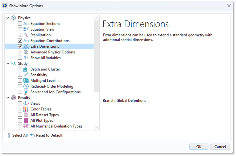 Enabling the Equation Contributions and Extra Dimensions checkboxes in the Show More Options dialog to access the features needed for manually defining the particle transport equation.
An extra dimension can then be added under Global Definitions, where its geometry and mesh are specified. Extra dimensions extend the standard model geometry by adding coordinates on which PDEs can be defined. In this case, an extra dimension may be one-, two-, or three-dimensional, depending on the geometry and the level of detail required for the particle model. Coupling operators, such as integration or averaging operators, can then be defined in the extra dimension to transfer information between the base geometry and the extra dimension, providing quantities for use in the governing equations and reaction kinetics, such as the average particle concentration or the concentration at the particle surface.
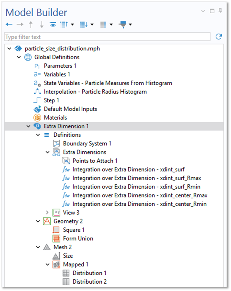
A two-dimensional extra dimension component representing the particle radial coordinate and particle size, together with its integration operators, geometry, and mesh.
After adding the extra dimension, the general workflow for manually defining the particle transport equation in the Lithium-Ion Battery interface is as follows. First, the Particle Properties setting in the Porous Electrode node is set to Nonintercalating particles. Setting this option disables the built-in particle diffusion formulation, allowing the particle transport equation to be defined manually. Two Weak Contribution nodes are then added to the Lithium-Ion Battery interface from the Equation Contributions submenu, which can be accessed by right-clicking the interface as shown in the screenshot below.
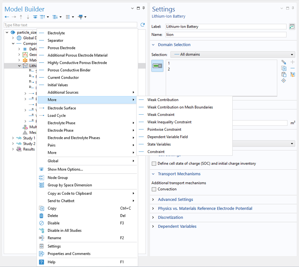 Accessing the Weak Contribution nodes from the More submenu of the Lithium-Ion Battery interface.
The Weak Contribution node defines the governing mass balance in the extra-dimensional domain. The particle concentration is introduced as an Auxiliary Dependent Variable under this node and serves as the dependent variable in the corresponding weak expression. The boundary Weak Contribution node defines the lithium flux boundary condition at the particle surface. The equations must be entered in weak form in the Settings window for each node.
When an extra dimension is included in the model, the settings for these Weak Contribution nodes enable them to be associated with geometric entities in that extra dimension by attaching to the corresponding domain in the physical geometry, as shown in the screenshot below.
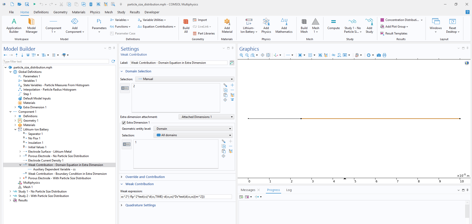 Settings window for the Weak Contribution node showing attachment to the extra dimension and the weak expression used to define the particle-transport domain equation in the particle-size distribution example.
The electrode reaction kinetics couple the solid-phase concentration variables to other variables in the DFN framework, including the electrolyte salt concentration, electrolyte potential, and solid-phase electric potential. To establish this coupling, as the last step, the Porous Electrode Reaction kinetics setting should be changed from the built-in Lithium insertion option to User defined. This allows either the exchange current density or the entire reaction current density expression to be specified using the manually defined particle concentration variable.
The Battery Electrode with a Particle Size Distribution example demonstrates this manual implementation approach. Rather than modifying the particle transport equation itself, the example extends the DFN framework by replacing the single-particle-size assumption with a particle-size distribution, allowing solid-phase intercalation to be modeled across a range of particle sizes.
In this example, the extra dimension is two-dimensional: one coordinate represents the radial position within a particle, while the other represents the particle-size range in the electrode. This formulation allows particle transport to be resolved across both the particle radius and the particle-size distribution. For a model with a single particle size, a one-dimensional extra dimension containing only the radial particle coordinate would be sufficient. The example compares cases with and without a particle-size distribution (screenshot below), providing a clear view of how the model setup changes when the built-in particle transport formulation in the Particle Intercalation node is replaced by a manually defined equation in an extra dimension.
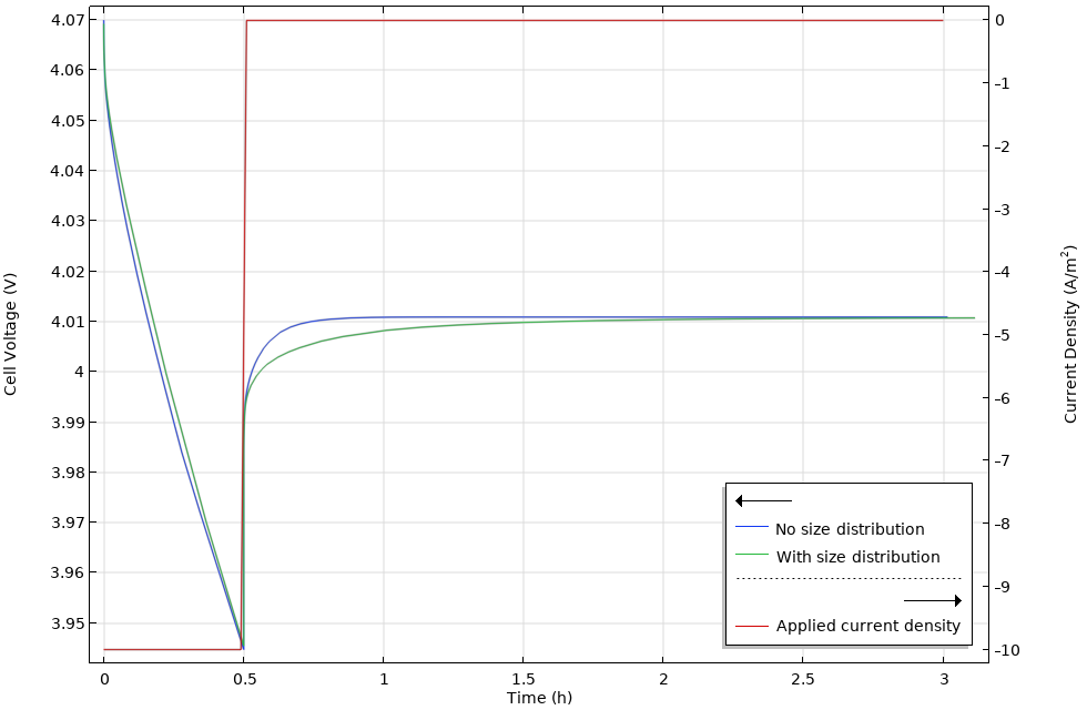 Cell voltage during a current pulse and the subsequent relaxation for cases with and without a particle-size distribution.
Although the discussion focused on customizing the particle transport equation within the DFN model underlying the Lithium-Ion Battery interface, the concepts presented are not limited to the particle diffusion equation, the DFN framework, or this particular physics interface. The following Nickel–Cadmium Battery example provides another useful case to review. In this model, a cylindrically symmetric extra dimension component is manually added to the Battery with Binary Electrolyte interface to represent proton diffusion within the nickel active material. This manual implementation is necessary in this case since the active material particles are modeled as cylinders with an inactive core. If the entire cylinders were active, the model could instead be configured using the standard Particle Intercalation node.
Conclusion
The ready-to-use battery modeling interfaces in COMSOL Multiphysics provide a convenient way to apply established modeling frameworks to a wide range of applications. At the same time, the predefined formulations can be adapted when a model requires additional detail or alternative physical descriptions. By understanding the underlying theory, locating the relevant equations in the physics interfaces, and becoming familiar with equation-based modeling, battery modelers can modify and extend existing formulations rather than build new models from scratch. This flexibility makes it possible to investigate new materials, mechanisms, and physical effects while retaining the structure and functionality of the built-in interfaces.



Comments (0)