Model Builder Features and Functionality

Operations, Sequences, and Selections

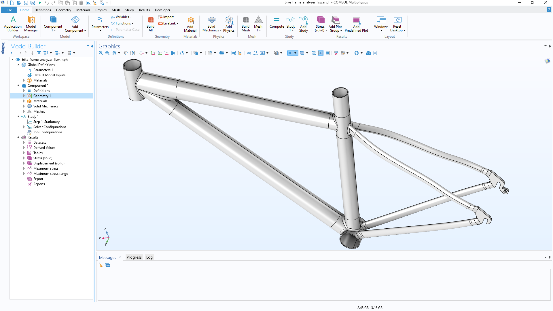
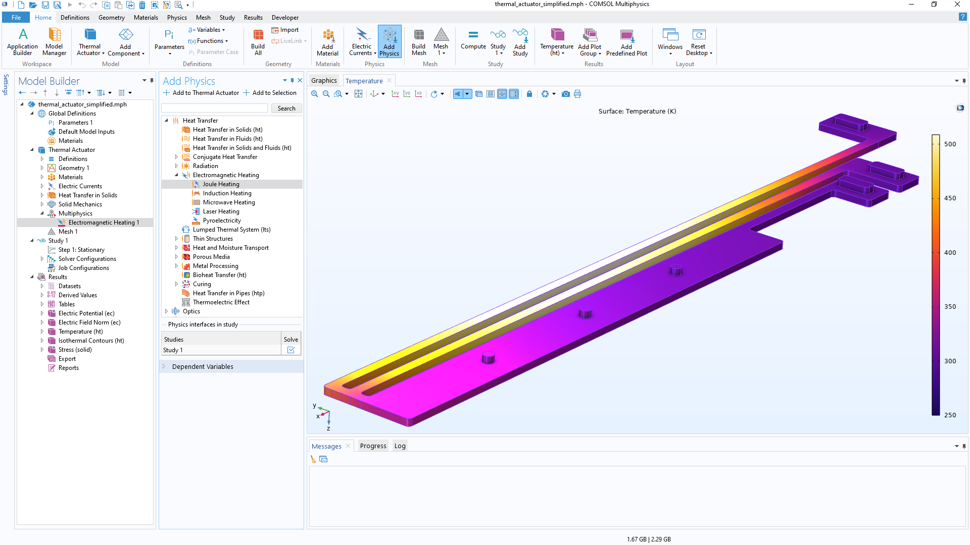
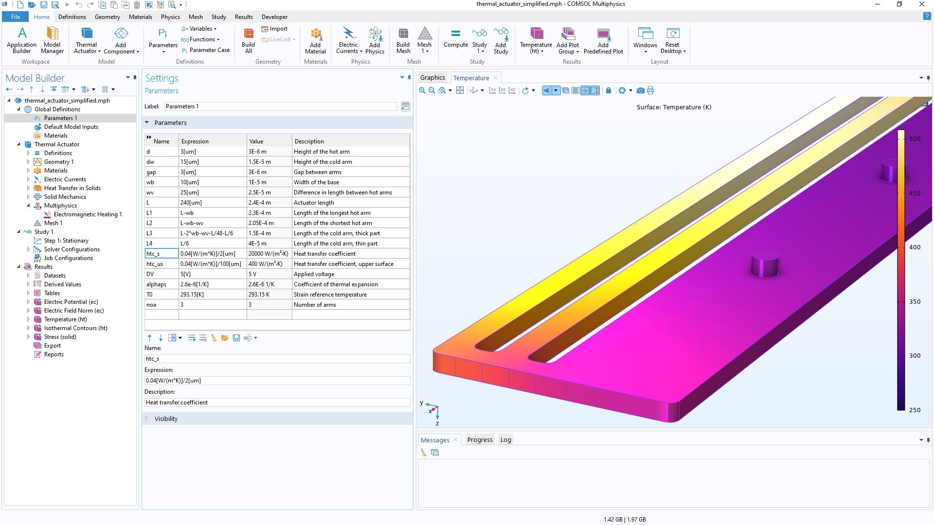
The core COMSOL Multiphysics^® package provides geometry modeling tools for creating parts using solid objects, surfaces, curves, and Boolean operations. Geometries are defined by sequences of operations, where each operation is able to receive input parameters for easy edits and parametric studies in multiphysics models. The connection between the geometry definition and defined physics settings is fully associative — a change in the geometry will automatically propagate related changes throughout the associated model settings.

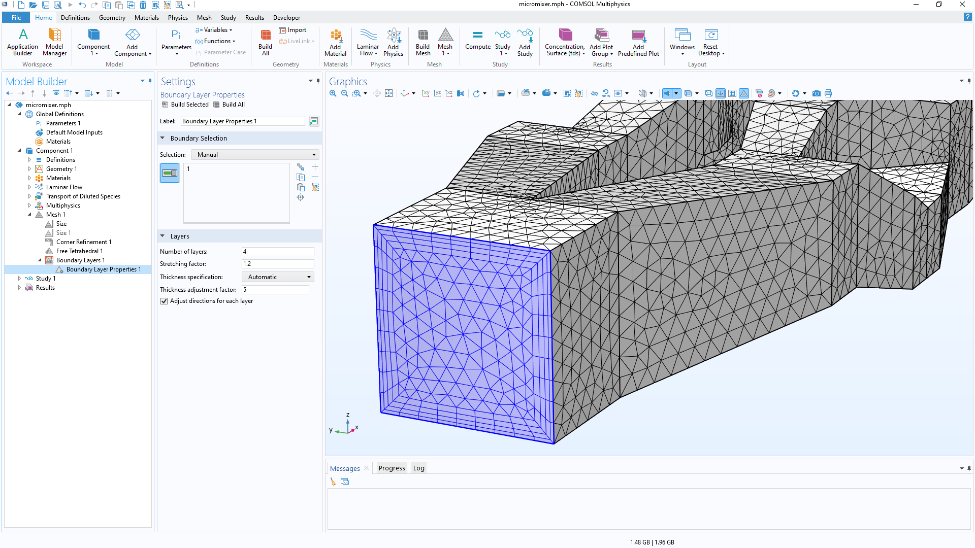
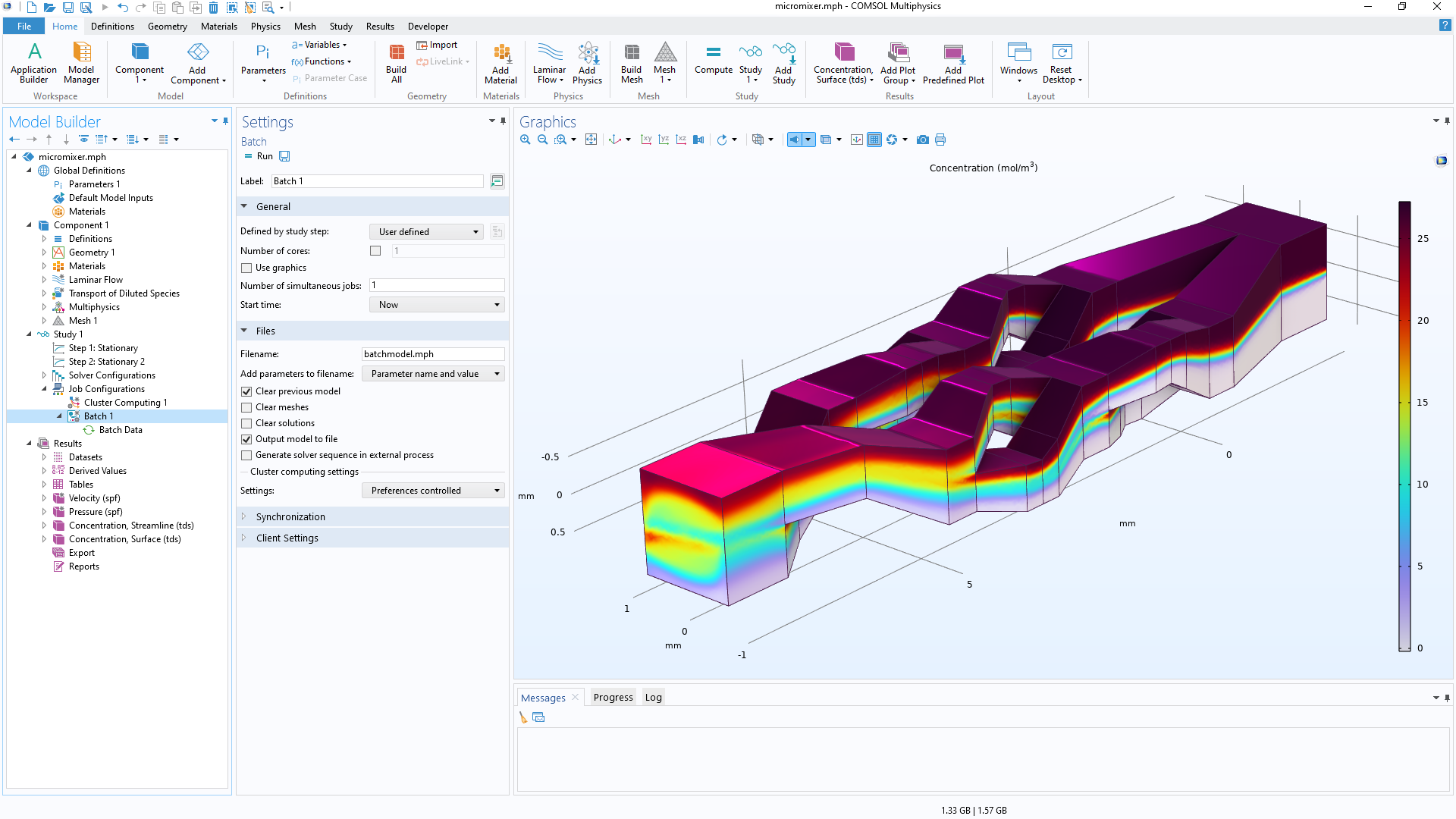
Geometric entities such as material domains and surfaces can be grouped into selections for subsequent use in physics definitions, meshing, and plotting. Additionally, a sequence of operations can be used to create a parametric geometry part, including its selections, which can then be stored in a Part Library for reuse in multiple models.

Import, Repair, Defeature, and Virtual Operations

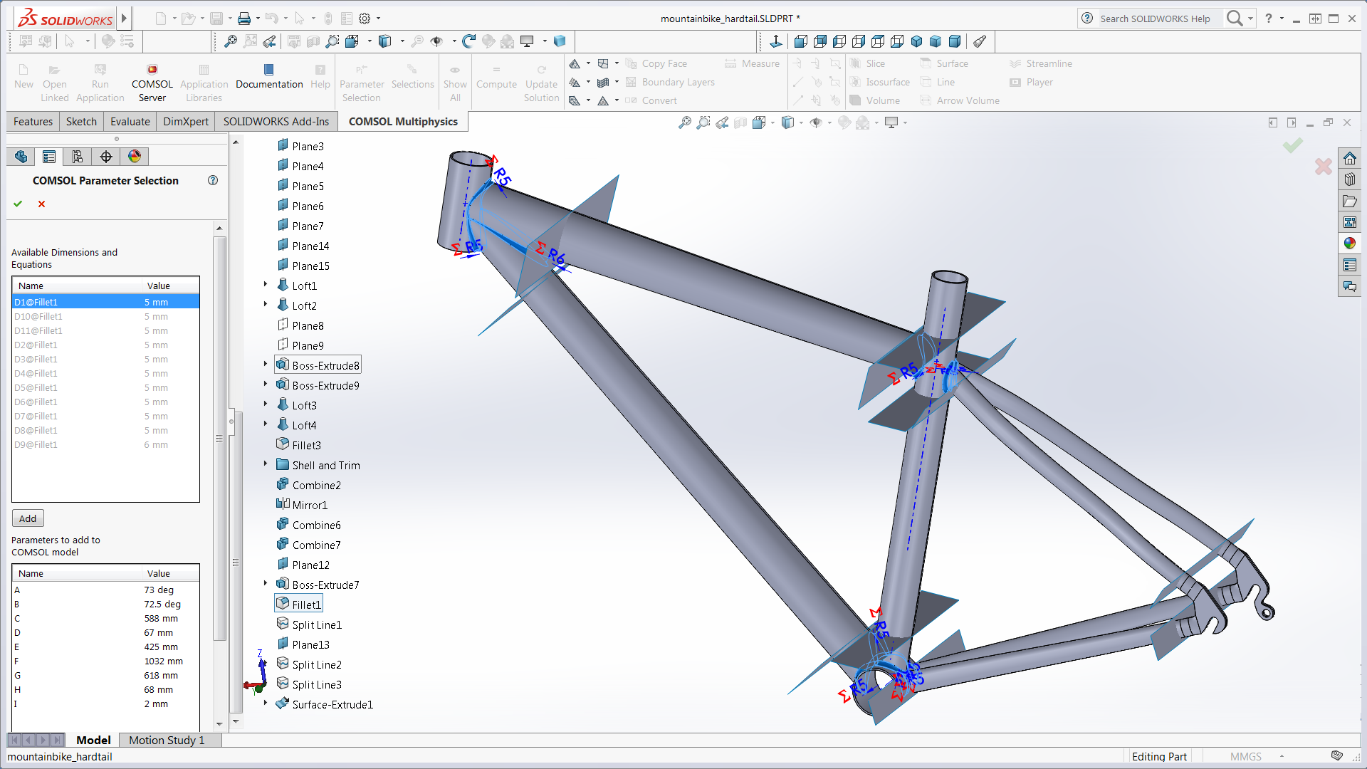
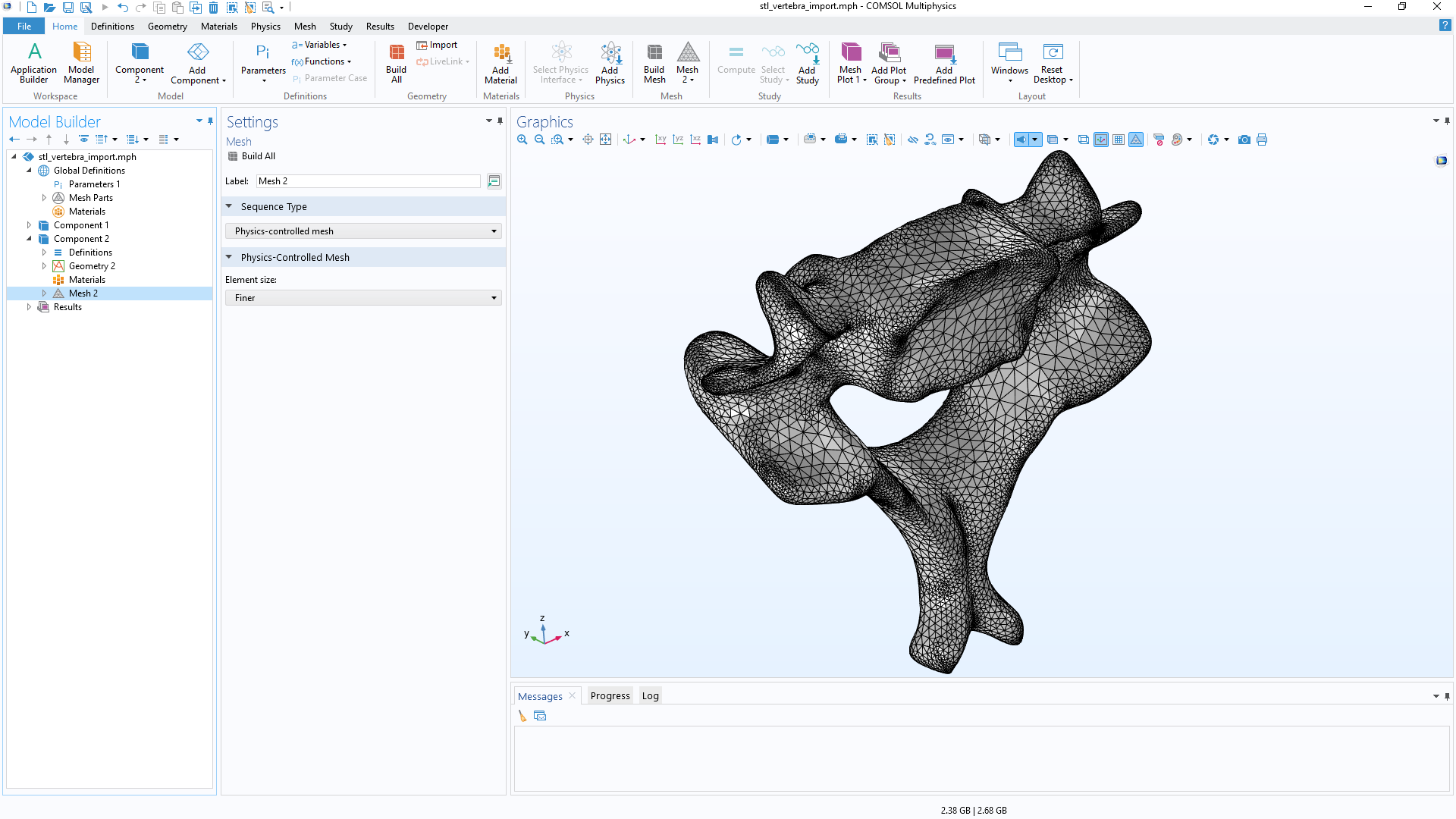
The import of all standard CAD and ECAD files into COMSOL Multiphysics^® is supported by the CAD Import Module and ECAD Import Module, respectively. The Design Module further extends the available geometry operations in COMSOL Multiphysics^®. Both the CAD Import Module and the Design Module provide the ability to repair and defeature geometries. Surface mesh models, such as in the STL format, can also be imported and then converted to a geometry object by the COMSOL Multiphysics^® core package. Import operations are like any other operation in the geometry sequence and can be used with selections and associativity for performing parametric and optimization studies.

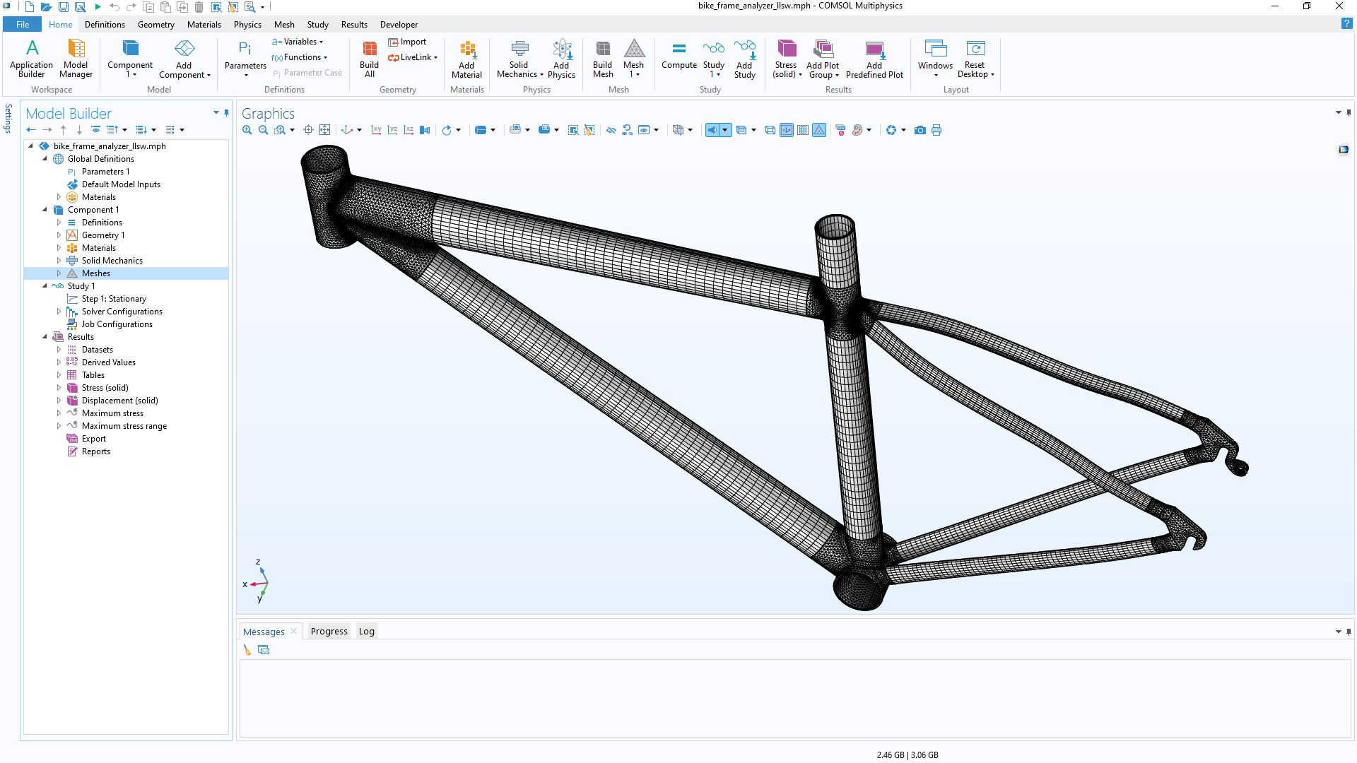
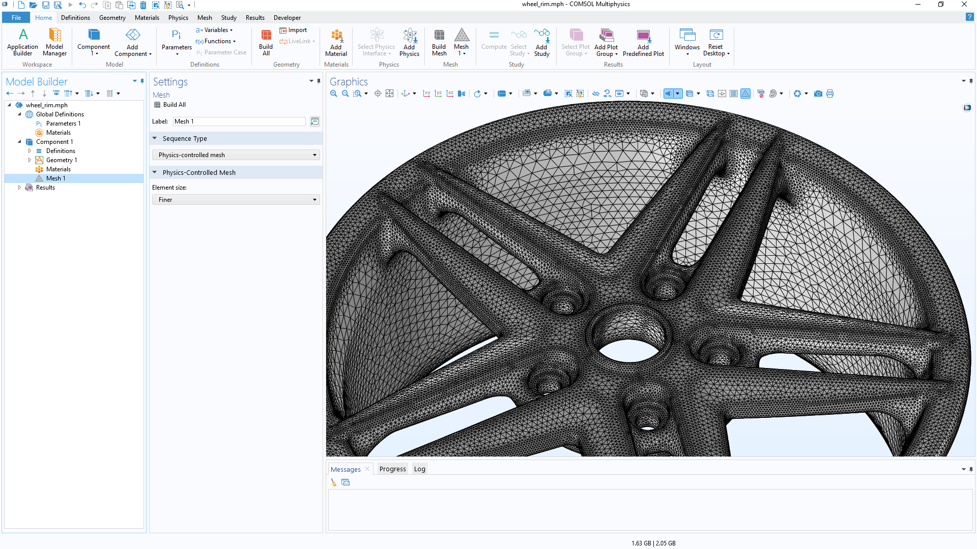
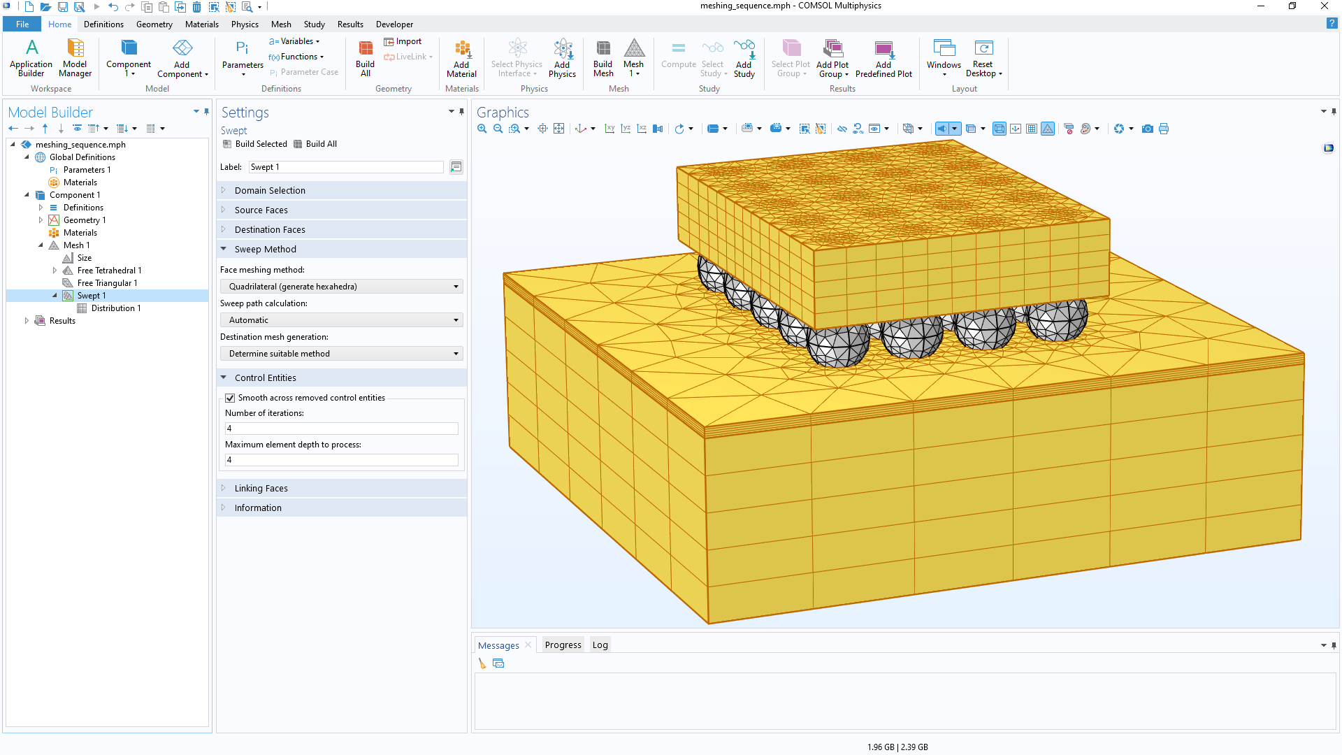
As an alternative to the defeature and repair capabilities of the COMSOL^® software, so-called virtual operations are also supported to eliminate the impact of artifacts on the mesh, such as sliver and small faces, which do not add to the accuracy of the simulation. In converse to defeaturing, virtual operations do not change the curvature or fidelity of the geometry, while yielding a cleaner mesh.

View a list of geometry modeling features

The COMSOL^® software contains predefined physics interfaces for modeling a wide range of physics phenomena, including many common multiphysics couplings. The physics interfaces are dedicated user interfaces for a particular scientific or engineering field, where all aspects for modeling the phenomena in question are made available for manipulation — from defining the model parameters to discretization to analyzing the results of the solution.

Upon selecting a particular physics interface, the software suggests available study types, such as time-dependent or stationary solvers. The software also automatically recommends the appropriate numerical discretization of the mathematical model, solver sequence, and visualization and postprocessing settings that are specific to the physics phenomena. The physics interfaces can also be combined freely in order to describe processes that involve multiple physics phenomena.

The COMSOL Multiphysics^® platform is preloaded with a large set of core physics interfaces for fields such as solid mechanics, acoustics, fluid flow, heat transfer, chemical species transport, and electromagnetics. By expanding the core package with add-on modules from the COMSOL^® product suite, you unlock a range of more specialized user interfaces that expand modeling capabilities within specific engineering fields.

View a list of physics-based modeling features

To really be useful for scientific and engineering studies and innovation, a software has to allow for more than just a hardwired environment. It should be possible to provide and customize your own model definitions based on mathematical equations directly in the user interface. The COMSOL Multiphysics^® software offers this level of flexibility with its built-in equation interpreter that can interpret expressions, equations, and other mathematical descriptions on the fly before it generates the numerical model. Adding and customizing expressions in the physics interfaces allows for freely coupling them with each other to simulate multiphysics phenomena.

The capabilities for customization go even further. With the Physics Builder, you can also use your own equations to create new physics interfaces for easy access and manipulation when you want to include them in future models or share them with colleagues.

View a list of equation-based modeling features

For discretizing and meshing your model, the COMSOL Multiphysics^® software uses different numerical techniques depending on the type of physics, or the combination of physics, that you are studying. The predominant discretization methods are finite-element based (for a more extensive list of methods, see the solvers section of this page). Accordingly, the general-purpose meshing algorithm creates a mesh with appropriate element types to match the associated numerical methods. For example, the default algorithm may use free tetrahedral meshing or a combination of tetrahedral and boundary-layer meshing, with a combination of element types, in order to provide faster and more accurate results.

For all of the mesh types, mesh refinement, remeshing, or adaptive meshing can be performed during the solution process or study step sequence.

View a list of meshing features

Study or Analysis Types

When you select a physics interface, a number of different studies (analysis types) are suggested by COMSOL Multiphysics^®. For example, for solid mechanics analyses, the software suggests time-dependent, stationary, or eigenfrequency studies; for CFD problems, the software would only suggest time-dependent and stationary studies. Other study types can also be freely selected for any analysis that you perform. Study step sequences structure the solution process to allow you to select the model variables for which you want to solve in each study step. The solution from any of the previous study steps can be used as input to a subsequent study step.

Sweeps, Optimization, and Estimations

Any study step can be run with a parametric sweep, which can include one or multiple parameters in a model, from geometry parameters to settings in the physics definitions. Sweeps can also be performed using different materials and their defined properties, as well as over lists of defined functions.

Optimization studies, using the Optimization Module, can be performed for topology optimization, shape optimization, or parameter estimations based on a multiphysics model. COMSOL Multiphysics^® offers both gradient-free and gradient-based methods for optimization. For parameter estimation, least-squares formulations and general optimization problem formulations are available. Built-in sensitivity studies are also available, where they compute the sensitivity of an objective function with respect to any parameter in the model.

View a list of studies

The equation interpreter in the COMSOL Multiphysics^® software delivers the best possible fuel to the numerical engine: the fully coupled system of PDEs for stationary (steady), time-dependent, frequency-domain, and eigenfrequency studies. The system of PDEs is discretized using the finite element method (FEM) for the space variables (x, y, z). For some types of problems, the boundary element method (BEM) can also be used to discretize space. For space- and time-dependent problems, the method of lines is used, where space is discretized with FEM (or BEM), thus forming a system of ordinary differential equations (ODEs). These ODEs are then solved using advanced methods, including implicit and explicit methods for time stepping.

Time-dependent and stationary (steady) problems can be nonlinear, also forming nonlinear equation systems after discretization. The engine in COMSOL Multiphysics^® delivers the fully coupled Jacobian matrix, which is the compass that points the nonlinear solver to the solution. A damped Newton method is used for solving the nonlinear system for stationary problems or during time stepping for time-dependent problems. The Newton method then solves a sequence of linear equation systems, using the Jacobian matrix, in order to find the solution to the nonlinear system.

For linear problems (also solved in the steps of the nonlinear solver, see above), the COMSOL^® software provides direct and iterative solvers. The direct solvers can be used for small- and midrange-sized problems, while the iterative solvers can be used for larger linear systems. The COMSOL^® software provides a number of iterative solvers with cutting-edge preconditioners, such as multigrid preconditioners. These preconditioners provide robustness and speed in the iterative solution process.

The different physics interfaces can also provide the solver settings with suggestions on the best possible default settings for a family of problems. These settings are not hardwired; you can change and manually configure the solver settings directly under each solver node in the user interface to tune the performance for your specific problem. When available, the solvers and other computationally intense algorithms are fully parallelized to make use of multicore and cluster computing. Both shared and distributed memory methods are available for direct and iterative solvers as well as for large parametric sweeps. All steps of the solution process can make use of parallel computing.

View a list of solvers

Show off your results to the world. COMSOL Multiphysics^® sports powerful visualization and postprocessing tools so that you can present your results in a meaningful and polished manner. You can use the built-in tools or expand your visualizations with derived physical quantities by entering mathematical expressions into the software. Therefore, you can visualize just about any quantity of interest related to your simulation results in COMSOL Multiphysics^®.

Visualization capabilities include surface, slice, isosurface, cut plane, arrow, and streamline plots, to name just a few plot types. A range of numerical postprocessing tools are available for evaluation of expressions, such as integrals and derivatives. You can compute the max, min, average, and integrated values of any quantity or derived quantities throughout volumes, on surfaces, along curved edges, and at points. Postprocessing tools specific to certain areas of engineering and science have also been included in many of the physics-based modules.

Exporting Results and Generating Reports with Other Software

You can export data and process it via third-party tools. Numerical results can be exported to text files on the .txt, .dat, and .csv formats as well as to the unstructured VTK format. With LiveLink™ for Excel^®, results can be exported to the Microsoft^® Excel^® spreadsheet software file format (.xlsx). Images can be exported to several common image formats, as well as the glTF™ file format for exporting 3D scenes. Animations can be exported in the WebM format and as animated GIF, Adobe^® Flash^® technology, or AVI files. Reports summarizing the entire simulation project can be exported to HTML (.htm, .html) or Microsoft^® Word^® software format (.doc).

View a list of results and postprocessing features