

The COMSOL Multiphysics® platform offers five add-on products for electrochemical modeling: the Battery Design Module, the Fuel Cell & Electrolyzer Module, the Corrosion Module, the Electrodeposition Module, and the Electrochemistry Module. Each module provides customized features and capabilities for specific applications of electrochemical systems. They also share something in common — a set of generic physics interfaces. In this blog post, we will focus on these shared interfaces. We will introduce the theory of current distribution, the corresponding physics interfaces, and guidelines for selecting an appropriate interface for a given application.
Table of Contents
- Selecting an Electrochemical Interface
- Primary, Secondary, and Tertiary Current Distribution Theory
- Physics Interfaces in the Electrochemistry Branch
- Summary of Physics Interface Assumptions
Selecting an Electrochemical Interface
The flow chart below can be used to provide guidance for selecting an interface. By considering which physical phenomena need to be resolved, including electrolyte mass transport, migration, electrode kinetics, and dissociation equilibria, as well as the assumptions that can be made about the electrolyte and electrode geometry, a suitable physics interface can be selected as a starting point. For each interface, the underlying theory is discussed in more detail, explaining the assumptions behind it.
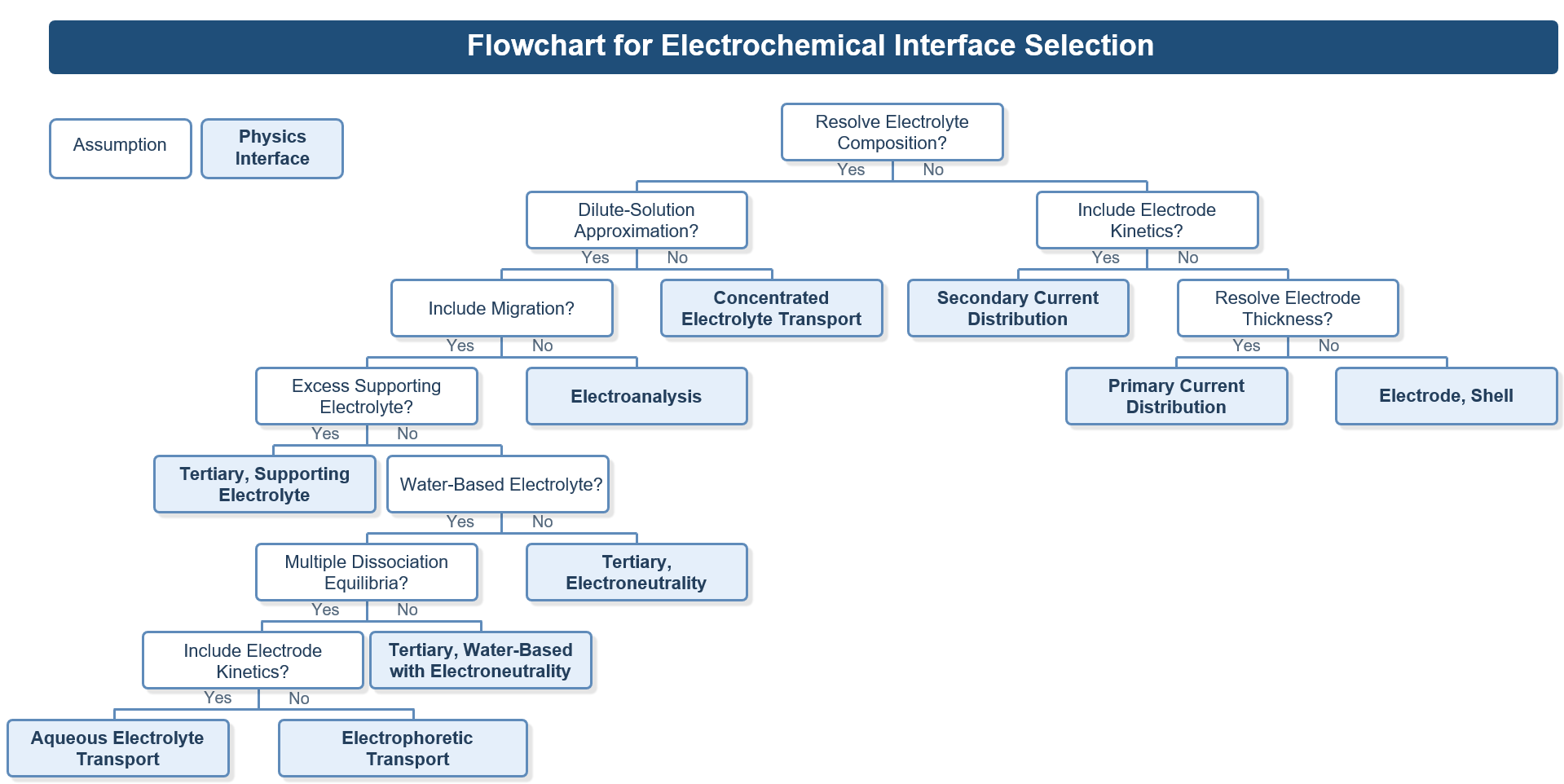 Flowchart for selecting an electrochemical interface.
In the following sections, the current distribution underlying each physics interface is introduced, along with representative examples of how to use the interface.
Primary, Secondary, and Tertiary Current Distribution Theory
Primary, secondary, and tertiary current distribution represent increasing levels of physical detail. Current distribution theory starts from charge conservation in the electronic conducting and electrolyte phases:
where \mathbf{i}_{\mathrm{s}} and \mathbf{i}_{\mathrm{l}} are the current densities in the electrode and electrolyte phases, and Q_{\mathrm{s}} and Q_{\mathrm{l}} are volumetric source or sink terms.
In primary and secondary current distributions, current conduction in both the electrode and electrolyte phases is described by Ohm’s law. The electrolyte composition is assumed to be uniform, and a constant electrolyte conductivity can be used. Current densities in the electrode and electrolyte phases are then written as:
where \sigma_{\mathrm{s}} and \sigma_{\mathrm{l}} are the conductivities of the electrode and electrolyte, and \phi_{\mathrm{s} and \phi_{\mathrm{l} are potentials in the electrode and electrolyte, respectively.
Primary Current Distribution Theory
In the primary current distribution, only ohmic losses in the electrochemical cell are considered, while electrode kinetics are neglected. Thus, no activation overpotential is considered, and the potential difference between the electrode and electrolyte is equal to the equilibrium potential, which can be expressed as:
Secondary Current Distribution Theory
In the secondary current distribution, electrode kinetics is included in addition to the ohmic effect. In this case, the local current density at the electrode–electrolyte interface is described as a function of the overpotential, which is the deviation of the electrode and electrolyte potential difference from the equilibrium potential:
The local current density i for an electrochemical reaction can be described using an appropriate kinetic expression, such as the Butler–Volmer equation:
where i_{\mathrm{0}} is the exchange current density, \alpha_{\mathrm{a} and \alpha_{\mathrm{c} are charge transfer coefficients, R is the universal gas constant, F is Faraday’s constant, and T is the temperature.
Tertiary Current Distribution Theory
In the tertiary current distribution, mass transport in the electrolyte is considered, and concentration gradients are no longer assumed to be negligible. The mass balance equation for each species i in the dilute electrolyte is given by the mass conservation equation:
where \mathbf{N}_{\mathrm{i}}, c_{\mathrm{i}}, and R_{\mathrm{i}} denote the total flux, concentration, and reaction source of species i, respectively. In the electrolyte, the total flux of species i can be expressed as:
where z_{\mathrm{i}} is the charge number, D_{\mathrm{i}} is the diffusion coefficient, u_{\mathrm{m},\mathrm{i}} is the mobility, and \mathbf{u} is the velocity field. The first, second, and third terms on the right-hand side represent diffusion, convection, and migration, respectively.
The electrolyte current density is then obtained by summing the contributions from all ionic species fluxes:
As a result, the electrolyte potential is solved for together with the species concentrations, rather than from Ohm’s law alone. This allows the effects of concentration gradients on ionic species transport to be accounted for in the current distribution. In tertiary current distribution, the electrolyte current is therefore influenced not only by conductivity and electrode kinetics, but also by changes in electrolyte composition.
Physics Interfaces in the Electrochemistry Branch
The assumptions underlying primary, secondary, and tertiary current distributions were introduced in the previous section. The interfaces in the Electrochemistry branch reflects the same progression, with different assumptions about current conduction, electrode kinetics, and mass transport in the electrolyte. In this section, these interfaces are introduced together with representative examples using each interface.
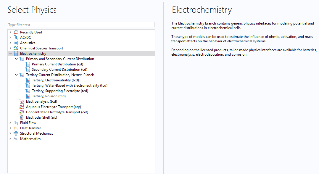 Physics interfaces in the Electrochemistry branch of the Select Physics window.
Primary Current Distribution Interface
The Primary Current Distribution interface is based on the theory of primary current distribution. It is used when the current distribution is governed mainly by ohmic effects and the cell geometry, and the influence of activation losses is neglected. The following model examples use this interface:
- Electrocoating of a Car Door
- Electrochemical Machining of a Microbore
- Primary Current Distribution in a Lead–Acid Battery Grid Electrode
Electrode, Shell Interface
The Electrode, Shell interface can be used for thin electrodes when the potential variations are in the direction normal to the electrode surface. Rather than explicitly resolving electrode thickness, the domain is replaced by a boundary equation that describes tangential current conduction. Current conduction in the shell electrode is described by Ohm’s law together with charge conservation. The following model example uses this interface:
Secondary Current Distribution Interface
The Secondary Current Distribution interface extends the Primary Current Distribution interface by including activation overpotentials through electrode kinetics. It can be used when electrode kinetics affect the current distribution, while mass transport in the electrolyte can be neglected. The following model examples use this interface:
- Current Distribution in a Chlor–Alkali Membrane Cell
- Decorative Plating
- Electroplating of a Printed Circuit Board
- Aluminum Anodization
- Anode Film Resistance Effect on Cathodic Corrosion Protection
- Galvanic Corrosion of a Magnesium Alloy in Contact with Steel
- Jelly Roll
- Jelly Roll Using a Flattened Geometry
Tertiary Current Distribution, Nernst–Planck Interface
As discussed, tertiary current distribution is used when mass transport in the electrolyte is no longer negligible and when concentration gradients influence the current distribution. The Tertiary Current Distribution, Nernst–Planck interface accounts for these effects by coupling ionic species transport to electrolyte charge conservation. The interface includes five electrolyte charge-conservation models that describe coupled charge and mass transport in the electrolyte.
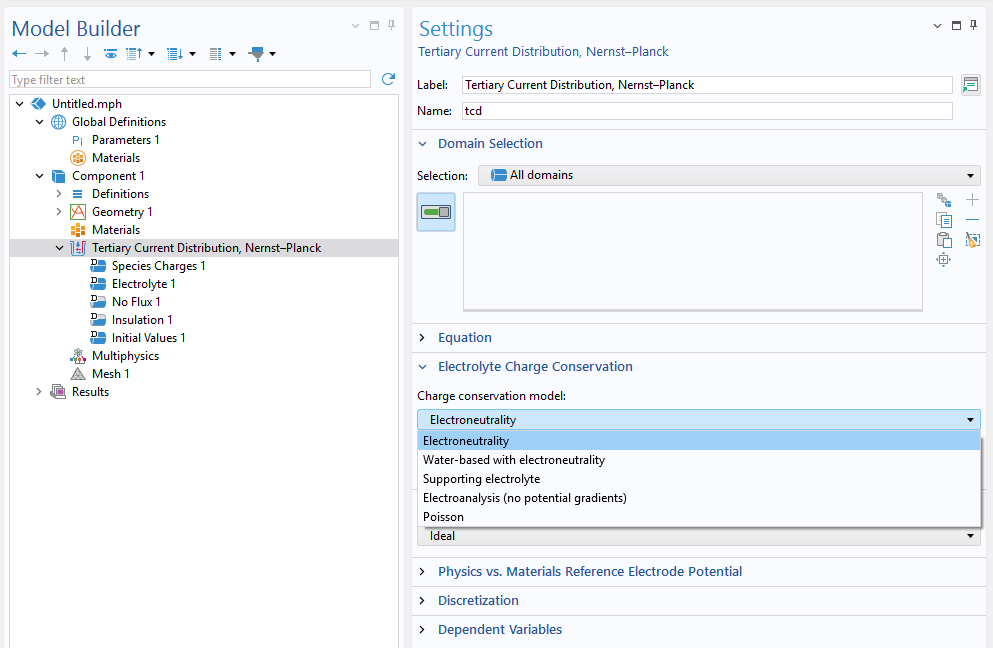 Charge conservation models.
Charge Conservation Model, Electroneutrality
The Electroneutrality option is used for systems with significant concentration gradients of ionic species. Under this assumption, the concentrations of the major ionic species are resolved explicitly, while local electroneutrality is imposed according to:
This is the general tertiary formulation for systems in which the major charge-carrying ions are included explicitly, and electroneutrality is assumed in the electrolyte. By combining the ionic flux expressions with the electroneutrality condition, the electrolyte current density can be expressed as:
where electrolyte conductivity \sigmacan be defined as: F^{2}\sum_{i=1}^{n} z_{i}^{2}u_{\mathrm{m},i}c_{i}
It is commonly used when concentration gradients are significant, and the main ionic species must be resolved directly. The following model examples use this option:
- Electrochemical Treatment of Tumors
- Capacitive Deionization of Saline Water
- Desalination in an Electrodialysis Cell (Ion-exchange membrane)
- Corrosion Inhibitor Transport
- Lithium Sulfur
- Vanadium Redox Flow Battery
- Electrochemical capacitor with porous electrode
Charge Conservation Model, Water-Based with Electroneutrality
The Water-based with electroneutrality option extends the electroneutrality option by incorporating the water auto-ionization equilibrium reaction for aqueous electrolyte. It accounts for proton and hydroxide ion transport, allowing the local pH to be calculated from proton concentration. The following model examples use this option:
Charge Conservation Model, Supporting Electrolyte
The Supporting electrolyte option can be used when the system contains a strong or well-mixed supporting electrolyte so that most of the concentration of charge-carrying species does not vary significantly. In this case, the electrolyte conductivity may also be treated as constant. The following model examples use this option:
An equivalent implementation of the Tertiary, Supporting electrolyte option can be obtained by coupling the Secondary Current Distribution interface with the Transport of Diluted Species interface from the Chemical Species Transport branch. The following model examples use this implementation:
Charge Conservation Model, Poisson
The Poisson option can be used when local electroneutrality is not assumed, and the potential in the electrolyte is obtained from Poisson’s equation. It can be used in cases where charge-separation effects are of interest, typically within a few nanometers of an electrode surface. The following example models use this option:
Charge Conservation Model, Electroanalysis
The Electroanalysis option can be used for electroanalytical problems in electrolytes containing a large excess of inert supporting electrolyte. Under this assumption, the conductivity is high enough that ohmic losses can be neglected. In addition, the electrolyte potential is not solved, and the migration effect is neglected. The transport of ionic species is described mainly by diffusion, with convection included when needed. The following model examples use this option:
- Cyclic Voltammetry at a Macroelectrode in 1D
- Electrochemical Impedance Spectroscopy
- Voltammetry at a Microdisk Electrode
- Alternating Current-Induced Corrosion
- Adsorption–Desorption Voltammetry
- Glucose Sensor
- Thin Layer Chronoamperometry
The Electroanalysis option can be either chosen from the Tertiary Current Distribution, Nernst–Planck interface or directly chosen as a physics interface from the Electrochemistry branch when adding physics.
Aqueous Electrolyte Transport Interface
The Aqueous Electrolyte Transport interface can be used for aqueous systems containing weak acids, weak bases, ampholytes, and complex species. It is based on the same assumptions as the Tertiary Current Distribution, Nernst–Planck interface when the Water-based with electroneutrality option is selected. Due to its more efficient handling of multiple equilibrium reactions and easier model setup, the Aqueous Electrolyte Transport interface can be a more convenient choice in some cases than the Tertiary Current Distribution, Nernst–Planck interface, especially for applications such as atmospheric corrosion, mechanistic corrosion modeling, biological electrochemistry, and electrochemical sensor modeling. The following model examples use this interface:
- Accelerated Corrosion Test of a Scratched Galvanized Steel Sample
- Atmospheric Corrosion with Mass Transport
- Corrosion Under an Evans Droplet
- Crevice Corrosion of Iron in an Acetic Acid/Sodium Acetate Solution
- Carbon Dioxide Corrosion in Steel Pipes
- Pitting Corrosion in Stainless Steel
Electrophoretic Transport Interface
The Electrophoretic Transport interface can be used for water-based systems in which species transport is driven by electrolyte potential gradients, and electrode kinetics are not considered. This interface supports weak and strong acids and bases, ampholytes, proteins, and uncharged species. Transport is described by the Nernst–Planck equations together with electroneutrality, dissociation equilibria, and water auto-ionization. Compared with the Aqueous Electrolyte Transport interface, it is tailored to electrophoresis applications. The following model examples use this interface:
This interface can be added from the Chemical Species Transport branch.
Concentrated Electrolyte Transport Interface
The electrolyte transport formulations discussed so far are based on dilute-solution theory. The Concentrated Electrolyte Transport interface can be used when the electrolyte needs to be modeled as a concentrated solution, with transport governed by the Maxwell–Stefan diffusion equation assuming local electroneutrality. In contrast to the Nernst–Planck equations, the concentrated solution theory does not assume that the electrolyte species are diluted in a neutral solvent of constant concentration. Typical electrolytes that can be modeled include ionic liquids, molten salts, and highly concentrated solutions. More theory is discussed in the blog post Introduction to the Concentrated Electrolyte Transport Interface. The following model example uses this interface:
The Electrochemistry branch includes interfaces at different levels of electrochemical modeling, from generic current-distribution interfaces to specialized interfaces for different types of electrochemical applications.
Summary of Physics Interface Assumptions
The interfaces discussed above use different assumptions for current distribution, electrolyte transport, and electrolyte description. The table below summarizes the main assumptions and formulations associated with each interface. A check mark indicates that the corresponding physical effect, assumption, or transport formulation is included in the interface. A blank indicates that it is not part of the default formulation or is not applicable.
|
Physics Interface |
Ohmic Losses |
Electrode Kinetics |
Mass Transport |
Electroneutrality |
Water-Based Electrolyte |
Dilute Electrolyte |
Concentrated Electrolyte |
|---|---|---|---|---|---|---|---|
|
Primary Current Distribution |
\checkmark |
||||||
|
Electrode, Shell |
\checkmark |
||||||
|
Secondary Current Distribution |
\checkmark |
\checkmark |
|||||
|
Tertiary, Electroneutrality |
\checkmark |
\checkmark |
\checkmark |
\checkmark |
\checkmark |
||
|
Tertiary, Water-Based with Electroneutrality |
\checkmark |
\checkmark |
\checkmark |
\checkmark |
\checkmark |
\checkmark |
|
|
Tertiary, Supporting Electrolyte |
\checkmark |
\checkmark |
\checkmark |
\checkmark |
|||
|
Tertiary, Poisson |
\checkmark |
\checkmark |
\checkmark |
\checkmark |
|||
|
Electroanalysis |
\checkmark |
\checkmark |
\checkmark |
||||
|
Aqueous Electrolyte Transport |
\checkmark |
\checkmark |
\checkmark |
\checkmark |
\checkmark |
\checkmark |
|
|
Electrophoretic Transport |
\checkmark |
\checkmark |
\checkmark |
\checkmark |
\checkmark |
||
|
Concentrated Electrolyte Transport |
\checkmark |
\checkmark |
\checkmark |
\checkmark |
\checkmark |
Specification chart of generic electrochemical interfaces.
The interfaces discussed in this blog post provide a starting point for building electrochemical models in COMSOL Multiphysics®. They span different assumptions, levels of detail, and application areas. The interface that is chosen helps define the scope of the model from the beginning and determines how current distribution, electrode kinetics, and species transport are represented. It also provides the basis for extending the model to include additional physical effects or multiphysics couplings.





Comments (0)