
Today, guest blogger René Christensen of GN Hearing discusses including thermoviscous losses in the topology optimization of microacoustic devices.
Topology optimization helps engineers design applications in an optimized manner with respect to certain a priori objectives. Mainly used in structural mechanics, topology optimization is also used for thermal, electromagnetics, and acoustics applications. One physics that was missing from this list until last year is microacoustics. This blog post describes a new method for including thermoviscous losses for microacoustics topology optimization.
Standard Acoustic Topology Optimization
A previous blog post on acoustic topology optimization outlined the introductory theory and gave a couple of examples. The description of the acoustics was the standard Helmholtz wave equation. With this formulation, we can perform topology optimization for many different applications, such as loudspeaker cabinets, waveguides, room interiors, reflector arrangements, and similar large-scale geometries.
The governing equation is the standard wave equation with material parameters given in terms of the density \rho and the bulk modulus K. For topology optimization, the density and the bulk modulus are interpolated via a variable, \epsilon. This interpolation variable ideally takes binary values: 0 represents air and 1 represents a solid. During the optimization procedure, however, its value follows an interpolation scheme, such as a solid isotropic material with penalization model (SIMP), as shown in Figure 1.
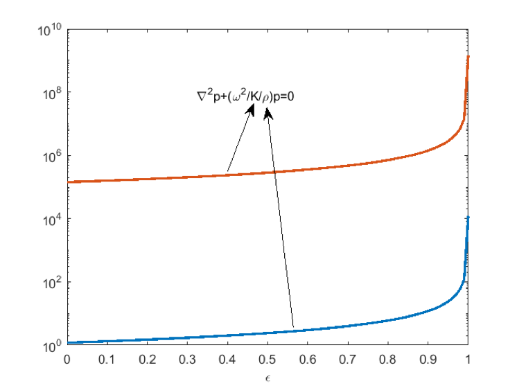
Figure 1: The density and bulk modulus interpolation for standard acoustic topology optimization. The units have been omitted to have both values in the same plot.
Using this approach will work for applications where the so-called thermoviscous losses (close to walls in the acoustic boundary layers) are of little importance. The optimization domain can be coupled to narrow regions described by, for example, a homogenized model (this is the Narrow Region Acoustics feature in the Pressure Acoustics, Frequency Domain interface). However, if the narrow regions where the thermoviscous losses occur change shape themselves, this procedure is no longer valid. An example is when the cross section of a waveguide changes shape.
Thermoviscous Acoustics (Microacoustics)
For microacoustic applications, such as hearing aids, mobile phones, and certain metamaterial geometries, the acoustic formulation typically needs to include the so-called thermoviscous losses explicitly. This is because the main losses occur in the acoustic boundary layer near walls. Figure 2 below illustrates these effects.
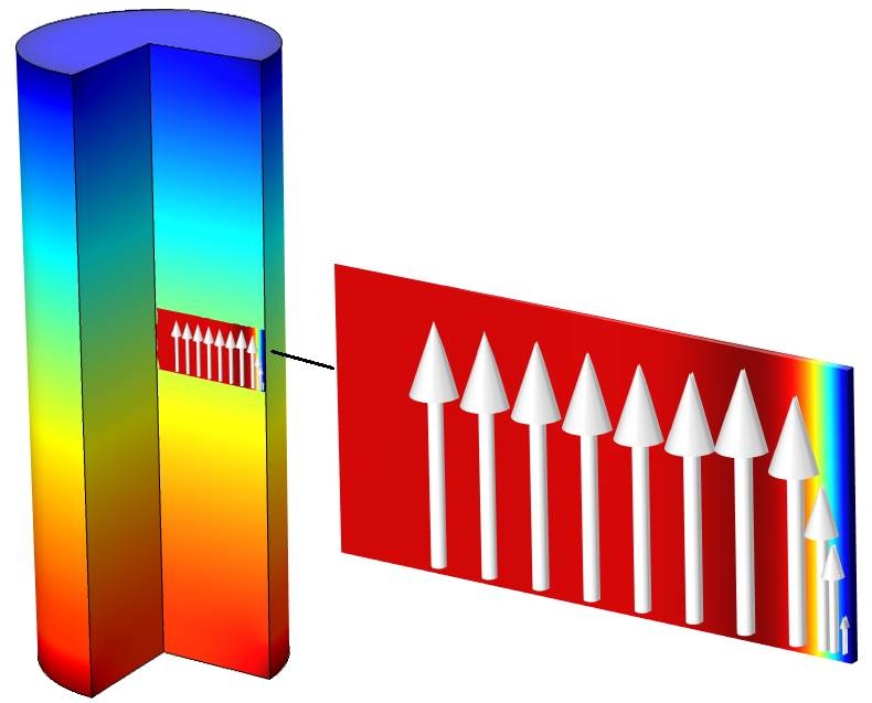
Figure 2: The volume field is the acoustic pressure, the surface field is the temperature variation, and the arrows indicate the velocity.
An acoustic wave travels from the bottom to the top of a tube with a circular cross section. The pressure is shown in a ¾-revolution plot.
The arrows indicate the particle velocity at this particular frequency. Near the boundary, the velocity is low and tends to zero on the boundary, whereas in the bulk, it takes on the velocity expected from standard acoustics via Euler’s equation. At the boundary, the velocity is zero because of viscosity, since the air “sticks” to the boundary. Adjacent particles are slowed down, which leads to an overall loss in energy, or rather a conversion from acoustic to thermal energy (viscous dissipation due to shear). In the bulk, however, the molecules move freely.
Governing Equations of Thermoviscous Acoustics
Modeling microacoustics in detail, including the losses associated with the acoustic boundary layers, requires solving the set of linearized Navier-Stokes equations with quiescent conditions. These equations are implemented in the Thermoviscous Acoustics physics interfaces available in the Acoustics Module add-on to the COMSOL Multiphysics® software. However, this formulation is not suited for topology optimization where certain assumptions can be used. A formulation based on a Helmholtz decomposition is presented in Ref. 1. The formulation is valid in many microacoustic applications and allows decoupling of the thermal, viscous, and compressible (pressure) waves. An approximate, yet accurate, expression (Ref. 1) links the velocity and the pressure gradient as
where the viscous field \Psi_{v} is a scalar nondimensional field that describes the variation between bulk conditions and boundary conditions.
In the figure above, the surface color plot shows the acoustic temperature variation. The variation on the boundary is zero due to the high thermal conductivity in the solid wall, whereas in the bulk, the temperature variation can be calculated via the isentropic energy equation. Again, the relationship between temperature variation and acoustic pressure can be written in a general form (Ref. 1) as
where the thermal field \Psi_{h} is a scalar, nondimensional field that describes the variation between bulk conditions and boundary conditions.
As will be shown later, these viscous and thermal fields are essential for setting up the topology optimization scheme.
Topology Optimization for Thermoviscous Acoustics Applications
For thermoviscous acoustics, there is no established interpolation scheme, as opposed to standard acoustics topology optimization. Since there is no one-equation system that accurately describes the thermoviscous physics (typically, it requires three governing equations), there are no obvious variables to interpolate. However, I will describe a novel procedure in this section.
For simplicity, we look at only wave propagation in a waveguide of constant cross section. This is equivalent to the so-called Low Reduced Frequency model, which may be known to those working with microacoustics. The viscous field can be calculated (Ref. 1) via Equation 1 as
(1)
where \Delta_{cd} is the Laplacian in the cross-sectional direction only. For certain simple geometries, the fields can be calculated analytically (as done in the Narrow Region Acoustics feature in the Pressure Acoustics, Frequency Domain interface). However, when used for topology optimization, they must be calculated numerically for each step in the optimization procedure.
In standard acoustics topology optimization, an interpolation variable varies between 0 and 1, where 0 represents air and 1 represents a solid. To have a similar interpolation scheme for the thermoviscoacoustic topology optimization, I came up with a heuristic approach, where the thermal and viscous fields are used in the interpolation strategy. The two typical boundary conditions for the viscous field (Ref. 1) are
and
These boundary conditions give us insight into how to perform the optimization procedure, since an air-solid interface could be represented by the former boundary condition and an air-air interface by the latter. We write the governing equation in a more general matter:
We already know that for air domains, (av,fv) = (1,1), since that gives us the original equation (1). If we instead set av to a large value so that the gradient term becomes insignificant, and set fv to zero, we get
This corresponds exactly to the boundary condition for no-slip boundaries, just as a solid-air interface, but obtained via the governing equation. We need this property, since we have no way of applying explicit boundary conditions during the optimization. So, for solids, (av,fv) should have values of (“large”,0). Thus, we have established our interpolation extremes:
and
I carried out a comparison between the explicit boundary conditions and interpolation extremes, with the test geometry shown in Figure 3. On the left side, boundary conditions are used, whereas on the adjacent domains on the right, the suggested values of av and fv are input.
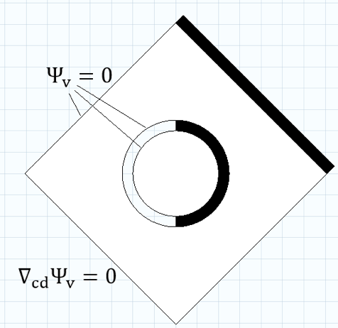
Figure 3: On the left, standard boundary conditions are applied. On the right, black domains indicate a modified field equation that mimics a solid boundary. White domains are air.
The field in all domains is now calculated for a frequency with a boundary layer thick enough to visually take up some of the domain. It can be seen that the field is symmetric, which means that the extreme field values can describe either air or a solid. In a sense, that is comparable to using the actual corresponding boundary conditions.
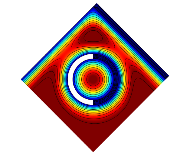
Figure 4: The resulting field with contours for the setup in Figure 3.
The actual interpolation between the extremes is done via SIMP or RAMP schemes (Ref. 2), for example, as with the standard acoustic topology optimization. The viscous field, as well as the thermal field, can be linked to the acoustic pressure variable pressure via equations. With this, the world’s first acoustic topology optimization scheme that incorporates accurate thermoviscous losses has come to fruition.
Optimizing an Acoustic Loss Response
Here, we give an example that shows how the optimization method can be used for a practical case. A tube with a hexagonally shaped cross section has a certain acoustic loss due to viscosity effects. Each side length in the hexagon is approximately 1.1 mm, which gives an area equivalent to a circular area with a radius of 1 mm. Between 100 and 1000 Hz, this acoustic loss increases by a factor of approximately 2.6, as shown in Figure 7. Now, we seek to find an optimal topology so that we obtain a flatter acoustic loss response in this frequency range, with no regards to the actual loss value. The resulting geometry looks like this:
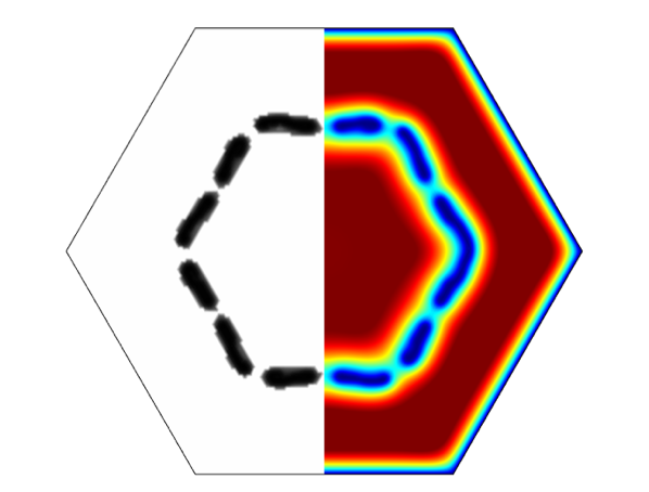
Figure 5: The topology for a maximally flat acoustic loss response and resulting viscous field at 1000 Hz.
A simpler geometry that resembles the optimized topology was created, where explicit boundary conditions can be applied.
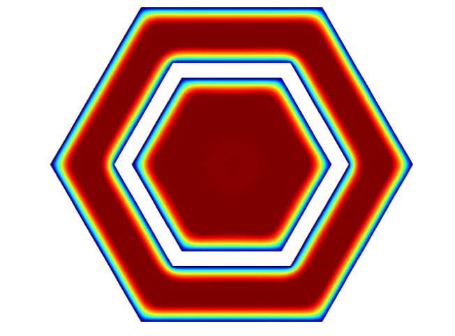
Figure 6: A simplified representation of the optimized topology, with the viscous field at 1000 Hz.
The normalized acoustic loss for the initial hexagonal geometry and the topology-optimized geometry are compared in Figure 7. For each tube, the loss is normalized to the value at 100 Hz.
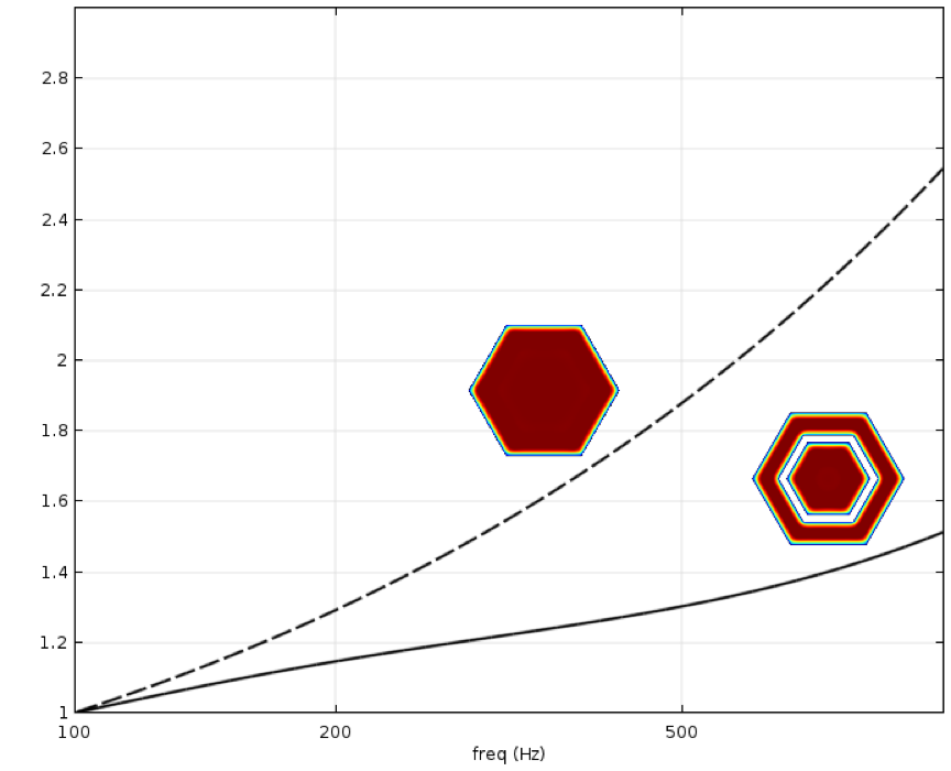
Figure 7: The acoustics loss normalized to the value at 100 Hz for the initial cross section (dashed) and the topology-optimized geometry (solid), respectively.
For the optimized topology, the acoustic loss at 1000 Hz is only 1.5 times higher than at 100 Hz, compared to the 2.6 times for the initial geometry. The overall loss is larger for the optimized geometry, but as mentioned before, we do not consider this in the example.
This novel topology optimization strategy can be expanded to a more general 1D method, where pressure can be used directly in the objective function. A topology optimization scheme for general 3D geometries has also been established, but its implementation is still ongoing. It would be very advantageous for those of us working with microacoustics to focus on improving topology optimization, in both universities and industry. I hope to see many advances in this area in the future.
References
- W.R. Kampinga, Y.H. Wijnant, A. de Boer, “An Efficient Finite Element Model for Viscothermal Acoustics,” Acta Acoustica united with Acoustica, vol. 97, pp. 618–631, 2011.
- M.P. Bendsoe, O. Sigmund, Topology Optimization: Theory, Methods, and Applications, Springer, 2003.
About the Guest Author
René Christensen has been working in the field of vibroacoustics for more than a decade, both as a consultant (iCapture ApS) and as an engineer in the hearing aid industry (Oticon A/S, GN Hearing A/S). He has a special interest in the modeling of viscothermal effects in microacoustics, which was also the topic of his PhD. René joined the hardware platform R&D acoustics team at GN Hearing as a senior acoustic engineer in 2015. In this role, he works with the design and optimization of hearing aids.


Comments (0)