
Hearing aids, mobile phones, and headphones require quality sound production to optimize a user’s experience. To evaluate the performance of a design, audio engineers create prototypes with a head and torso simulator (HATS), a manikin that mimics the hearing environment of an adult human. For a more cost-efficient approach, one option is simulating this setup via the COMSOL® software in order to perform virtual acoustic measurements.
Measuring the Performance of Acoustic Devices for the Human Ear
When developing products such as hearing aids and headphones, an important factor is testing the sound quality for human perception. However, using a subjective experience to collect measurements of binaural analyses can present challenges such as reverberation, because human interaction with sound is very complex. To measure the overall sound quality of various acoustic products, audio engineers use HATS to realistically reproduce the acoustic behavior of a human.
HATS are manufactured manikins with built-in ear and mouth simulators that provide realistic acoustic properties of an average adult human head and torso to test products for improvements and additional functionality. These manikins are designed to carry out in situ electroacoustics measurements for accurate 3D testing in a standardized way. To perform repetitive tests and achieve faster results, engineers can combine this design environment with numerical simulation.
With the COMSOL Multiphysics® software and add-on Acoustics Module, you can construct a mathematical model for head and torso simulators directly in the software using the boundary element method (BEM). With the features included in the module, it’s possible to create virtual prototypes for acoustic applications that are not only cost-efficient, but also provide the details and validation of binaural analyses in a more timely matter.
An example of a 3D HATS simulation, SPL for varying frequencies. The higher the frequency, the more cancellations are visualized.
Modeling a Head and Torso Simulator with the Boundary Element Method
In this example of a HATS, most of the model geometry is generic, while only the ears are based on a 3D scan of an actual human. Two microphones are positioned at the entrances of the ear canals. This generic geometry represents the entire upper body and contains all the acoustic aspects of a human being, such as the auditory canal and mouth cavity.
This model uses BEM and the Pressure Acoustics, Boundary Elements interface to analyze the acoustic field in the half space domain exterior of a generic HATS, as if it were standing on a table. When modeling with acoustics and solving for exterior problems like this one, using BEM is significantly easier and faster compared to the finite element method (FEM) in that it only uses mesh elements on the boundaries of the modeled regions. Because this model uses BEM, there is an infinite void used that represents a single unbounded region surrounding the manikin. To model scattering problems, a Background Pressure Field feature is applied to model a plane wave propagating toward the manikin.
This example also uses two Physiological impedance boundary conditions with the Human Ear without Pinna option, shown in the figure below to represent the left and right ear canal entrances. Physiological models contain experimentally verified models of the human ear and human skin, which typically are of importance in acoustical applications. The impedance boundary condition is a good approximation for a locally reacting surface like this one, for which the normal velocity at any point depends only on the pressure at an exact point.
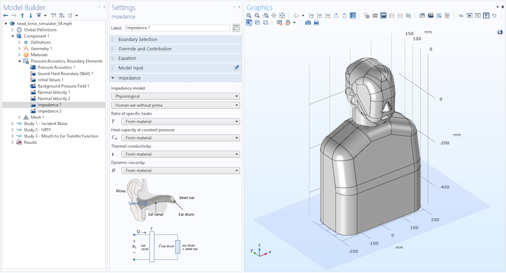
Example of the Physiological impedance boundary conditions used with the Human Ear without Pinna option, representing the ear canal entrances in the model.
You can use this model to analyze three different frequency domain studies:
- Incident wave analysis
- Head-related transfer function (HRTF)
- Mouth-to-ear transfer function
An incident wave analysis is used to model the scattering of a plane wave (propagating in a given direction) off the manikin, and the total and scattered sound pressure level (SPL) can be evaluated. An HRTF measures how sounds originating from different areas reach the ear — showing the diffraction and reflection properties of a sound wave from the source to the eardrum. The mouth-to-ear-transfer function is a more specific type of head-related transfer function. This study is performed by imposing a velocity at the mouth to compute the SPL at the ear canal entrance and the ear drum — where the difference between the input and output defines the transfer function.
Evaluating Frequency Responses
Incident Wave Analysis
From the incident wave analysis results, we can view the total SPL (in the plot below) for a background pressure field propagating toward the manikin. The wave is propagating directly toward the front of the manikin. The plot shows that with the pressure applied, an SPL buildup occurs in front of the manikin (this is the classical pressure doubling). If you wanted to test a pair of headphones on the manikin, the sensitivity and SPL results can show how well the headphones are isolated from exterior excitation and noises. Be warned, though, that a continuous exposure to noise at or above 80 dB can result in hearing damage, so performing this type of analysis is important to find an appropriate power level when testing a pair of headphones.
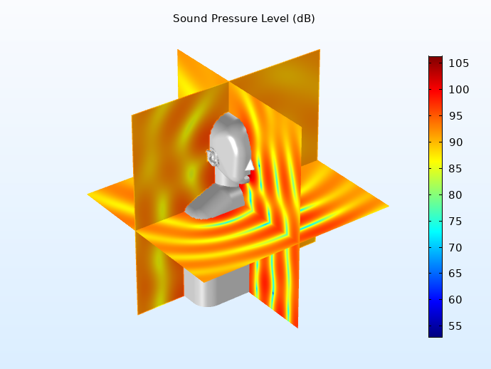
Total sound pressure level for the incident wave analysis.
The scattered acoustic pressure field for an off-axis incident wave can be seen in the image below. The angle of incidence of the plane wave can be modified in the model.
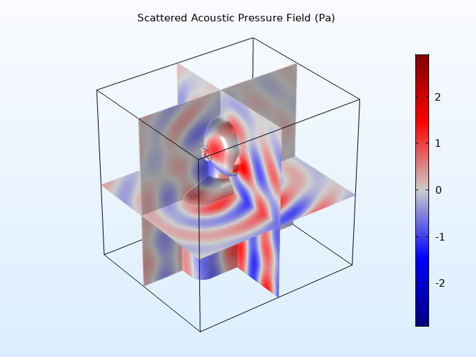
Scattered acoustic pressure field for the incident wave analysis.
HRTF
The polar group plot below, generated with the Radiation Pattern plot, shows the horizontal plane HRTF for the right ear of the HATS manikin. The results show that at higher frequencies, more complex patterns appear. Cancellation patterns and notches in the HRTF appear as the frequency increases and the wavelength decreases. The HRTF is computed using the reciprocity principle that allows us to interchange the source and receiver in pressure acoustics.
The source is placed at the ear canal entrance and the response is measured outside the manikin. In this way, we can obtain the full spatial HRTF for a single simulation (at a given frequency). The SPL and pressure plots below show the acoustic field for the source located at the ear canal entrance. This technique is not used in actual measurements, where the source is placed outside the head and the SPL is measured at the ear canal entrance with a probe microphone. This is because mimicking the measurement approach is expensive computationally, as one simulation needs to be done for each frequency and each direction.
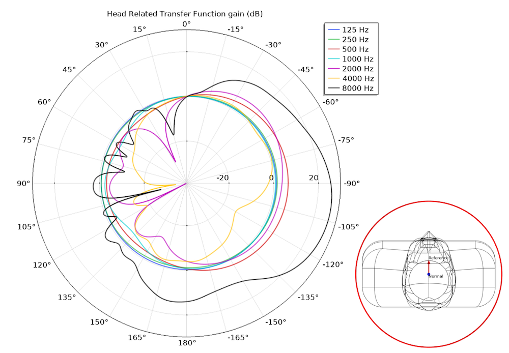
HRTF for a 1-meter radius at 125 Hz, 250 Hz, 500 Hz, 1000 Hz, 2000 Hz, 4000 Hz, and 8000 Hz.


Sound pressure level (left) and total acoustic pressure field (right) for the source placed at the ear canal entrance.
Mouth-to-Ear Transfer Function
The mouth-to-ear and the mouth-to-eardrum transfer functions are depicted in the graph below (only a coarse frequency resolution has been used here). The mouth-to-ear transfer function represents (to some extent) a system where a microphone is placed near the ear canal entrance and picks up a speech signal. The mouth-to-eardrum represents the full path from mouth to the auditory system. From the results, we can analyze the frequency response and see that the magnitude of the mouth-to-ear-canal entrance transfer function is less than that of the mouth-to-eardrum. The difference between the two transfer functions appear in the high frequency range, around 2000-3000 Hz, which is the typical location of the ear canal quarter wave resonance.
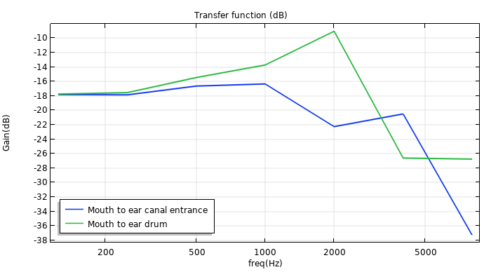
Mouth-to-ear-canal-entrance transfer function (blue) and mouth-to-eardrum transfer function (green).
From the acoustic pressure animation below, you can view how the sound pressure waves from the imposed velocity travel from the mouth to the ears.
An animation of the sound pressure waves traveling from the mouth to the ears.
By using the BEM functionality in COMSOL Multiphysics, you can achieve realistic acoustic measurements when testing the performance of your designs. This approach is less computationally expensive than FEM, allowing for faster and more efficient acoustic modeling simulations.
Next Steps
Try analyzing the acoustics of a head and torso simulator yourself by clicking the button below.


Comments (0)