

After solving a model in the COMSOL Multiphysics® software, we may want to fit the solution data to a set of functions defined in the simulation domain. In a previous blog post, we explained how to fit discrete empirical data to a curve, but here, we will instead consider the fitting of continuous solution data. We will then introduce the concept of orthogonality and explain how fitting the solution data to a set of orthogonal functions reduces to a simple and convenient postprocessing operation.
Benefits of Curve Fitting
In a previous blog post about fitting discrete experimental data, we explained how curve fitting can be useful for the ensuing simulation work. For example, if we try to use the raw experimental data to define a material property directly, then the statistical fluctuations in the data can make it more difficult for the solver to converge. Furthermore, fitting the discrete data to a smooth function provides access to higher-order derivatives of that function, whereas trying to numerically differentiate the raw data can be very noisy and error prone.
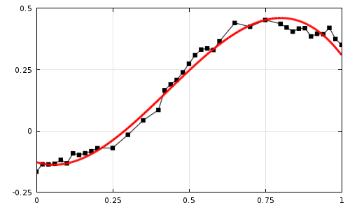
Raw experimental data (black dots) fit to a cubic polynomial (red curve).
What about curve fitting to the solution data from a previous study in the COMSOL Multiphysics model? One immediate benefit is data compaction. If we can find a linear combination of functions that gives good agreement with the full solution, then we can communicate much of the information from that full solution just by sharing the values of a few function coefficients. (Note that there is no one-size-fits-all strategy for data compaction; several other approaches, such as using probe tables and selections, are described in this Knowledge Base entry on reducing the amount of solution data stored in a model).
In addition, curve fitting of continuous solution data can be a convenient way to estimate the higher-order spatial derivatives of the solution. Many physics interfaces in the COMSOL® software use a finite element discretization consisting of piecewise Lagrange polynomials, which, by default, are often of the second degree. In this case, the derivatives are not necessarily continuous and third- or higher-order derivatives are always zero.
Overview of Least-Squares Fitting
Let us first look at the underlying mathematics of a simple least-squares fit. In some simulation domain (or a boundary or edge), which we denote by Ω, suppose that our COMSOL Multiphysics model has solved for a field variable u. Our goal is to approximate the value of u over this domain by treating it as a linear combination of a set of predefined functions,
where the fi are a set of known functions and the ci are coefficients that we must solve for.
A common way to determine these unknown coefficients is to take the L2 norm of the difference between u and its approximation,
and then to find values of ci corresponding to local minima of this L2 norm.
At a local minimum within Ω, the derivatives with respect to the unknown coefficients must equal zero,
where the subscript j is used to avoid confusion with the index of the summation.
Assuming that everything under the integral sign is sufficiently nice, by applying the chain rule, this simplifies to
Dropping the leading coefficient of 2 and swapping the order of the integration and discrete summation yields
This last result is a set of N linear equations for the N unknown coefficients. For example, if there are three polynomials, then we can write this result out in matrix form,
&\begin{bmatrix}
A_{11} & A_{12} & A_{13}\\
A_{21} & A_{22} & A_{23}\\
A_{31} & A_{32} & A_{33}
\end{bmatrix}
\begin{bmatrix}
c_1\\
c_2\\
c_3
\end{bmatrix}
=
\begin{bmatrix}
B_1\\B_2\\B_3\\
\end{bmatrix}\\
&A_{ij} \equiv \int_\Omega f_i(\mathbf{r})f_j(\mathbf{r})\textrm{d}\Omega
\qquad B_{j} \equiv \int_\Omega u(\mathbf{r})f_j(\mathbf{r})\textrm{d}\Omega
\end{aligned}
Therefore, solving this equation system for the unknown coefficients requires the evaluation of N(N+3)/2 integrals (noting that the matrix on the left-hand side is symmetric, i.e. the integral of fifj equals the integral of fjfi) and the solution of a set of N linear algebraic equations.
As we will see in the following sections, we can make the calculation of the coefficients ci significantly easier if we define the corresponding functions fi so that they are orthogonal in the region where we are trying to fit the solution data.
Introduction to Orthogonal Functions
In discussing the concept of orthogonality, we must be careful not to give an overly narrow definition. In general, two distinct vectors u and v belonging to a vector space are orthogonal under an inner product \langle u,v\rangle if \langle u,v\rangle = 0. The exact definition of the inner product can change depending on the vector space.
Since we are talking about curve fitting of a spatially varying solution vector to a set of functions f1(r), f2(r), … fN(r) in some region Ω of n-dimensional real coordinate space (\mathbf{r}\in\mathbb{R}^n), we can get more specific and define the inner product of these functions as
where w(r) is some yet-to-be-defined weight function, with the restriction that w(r) > 0 for all r in Ω.
For example, the functions f_1(x) = 1, f_2(x) = \sin x, and f_3(x) = \cos x are orthogonal under the inner product
That is, the region Ω is the one-dimensional interval x\in[-\pi,\pi] and the weight function is simply w(x)=1. We could prove the orthogonality of these functions by evaluating the integrals
\int_{-\pi}^\pi (1)^2 \textrm{d}x &= 2\pi \qquad \int_{-\pi}^\pi (\sin x)^2 \textrm{d}x = \pi \qquad \int_{-\pi}^\pi (\cos x)^2 \textrm{d}x = \pi \\
\int_{-\pi}^\pi (1)(\sin x) \textrm{d}x &= 0 \qquad \int_{-\pi}^\pi (1)(\cos x) \textrm{d}x = 0 \qquad\int_{-\pi}^\pi (\sin x)(\cos x) \textrm{d}x = 0\\
\end{aligned}
In fact, we could extend this concept further and see that the functions \sin(2x), \cos(2x), \sin(3x), \cos(3x), etc. are also orthogonal under the same inner product. The orthogonality of these trigonometric functions is the basis of Fourier series expansion.
Least-Squares Fitting with Orthogonal Functions
Now let us take what we know about orthogonal functions and revisit the linear least-squares fitting problem, which, as we saw earlier, reduces to solving for the set of coefficients ci such that
Now suppose that the functions fi are all orthogonal under the inner product
You might have noticed some sleight of hand: When talking about the inner product of an n-dimensional vector space, we have now used the differential element dΩ in the definition of the inner product, but dΩ will be expressed differently depending on our choice of coordinate system (such as Cartesian, cylindrical polar, spherical polar, etc.). As we will see in an example later on, for maximum convenience, we can choose a set of functions that are orthogonal under an inner product whose weight function equals the Jacobian determinant of the coordinate system being used.
Due to the orthogonality of the functions, all of the off-diagonal terms in the N \times N matrix on the left-hand side vanish, and now our set of N equations is now just a set of N expressions that give us the values of ci directly:
If we choose to normalize the functions such that the denominator of the above expression is one, we get the even simpler-looking expression
So the task of fitting the solution data to a set of N functions has been reduced to the task of evaluating N different integrals. In the COMSOL® software, you can easily define Integration couplings to evaluate an integral over any set of domains, boundaries, edges, or points in the geometry. (You do not even have to rerun the study after defining an Integration coupling; it is sufficient to just click Update Solution.)
In the remaining sections, we will look at a more practical example: fitting the deformation of a mirror to a set of Zernike polynomials.
The Zernike Polynomials
One of the most commonly used orthogonal functions in optics are the Zernike polynomials, which are functions of the radial coordinate and plane angle in a circle,
where
- ρ is the radial coordinate (0\leq\rho\leq 1)
- θ is the azimuthal angle (0\leq \theta < 2\pi)
- N_n^m is a normalization term
- R_n^{|m|}(\rho) is the radial term
- M(m\theta) is the meridional term or azimuthal term
- n is the radial index (n \in \left\{0,1,2,\dots\right\})
- m is the meridional or azimuthal index (for a given n, m \in \left\{-n, -n+2, -n+4, \dots , n-2, n\right\})
Note that there are several different standard formats for how the Zernike polynomials are defined and how their indices are interpreted. The function definitions used in COMSOL Multiphysics, which use two separate indices to describe the radial and azimuthal dependence of the functions, are consistent with ANSI and ISO standards (Refs. 1, 2). The Zernike polynomials are often defined with respect to a unit circle, but can then be defined on any other circle of radius R by replacing ρ with ρR (although this affects the normalization).
The first few Zernike polynomials are listed below.
| Term | Expression | Common Name |
|---|---|---|
| Z_0^0 | 1 | Piston |
| Z_1^{-1} | 2\rho \sin(\theta) | Vertical tilt |
| Z_1^1 | 2\rho \cos(\theta) | Horizontal tilt |
| Z_2^{-2} | \sqrt{6}\rho^2 \sin(2\theta) | Oblique astigmatism |
| Z_2^0 | \sqrt{3}\left(2\rho^2-1\right) | Defocus |
| Z_2^2 | \sqrt{6}\rho^2 \cos(2\theta) | Vertical astigmatism |
| Z_3^{-3} | \sqrt{8}\rho^3 \sin(3\theta) | Oblique trefoil |
| Z_3^{-1} | \sqrt{8}\left(3\rho^3-2\rho\right)\sin(\theta) | Vertical coma |
| Z_3^1 | \sqrt{8}\left(3\rho^3-2\rho\right)\cos(\theta) | Horizontal coma |
| Z_3^3 | \sqrt{8}\rho^3 \cos(3\theta) | Horizontal trefoil |
| Z_4^{-4} | \sqrt{10}\rho^4\sin(4\theta) | Oblique quadrafoil |
| Z_4^{-2} | \sqrt{10}\left(4\rho^4-3\rho^2\right)\sin(2\theta) | Oblique secondary astigmatism |
| Z_4^0 | \sqrt{5}\left(6\rho^4-6\rho^2+1\right) | Primary spherical |
| Z_4^2 | \sqrt{10}\left(4\rho^4-3\rho^2\right)\cos(2\theta) | Vertical secondary astigmatism |
| Z_4^4 | \sqrt{10}\rho^4\cos(4\theta) | Horizontal quadrafoil |
The normalization terms have been selected so that
where the Kronecker delta δ equals 1 if the two subscripts are equal or 0 otherwise.
In keeping with our earlier terminology, the Zernike polynomials are orthogonal on the unit circle under the weight function w(\rho,\theta)=\rho. It is convenient that the weight function ρ happens to exactly match the Jacobian determinant when converting between Cartesian and cylindrical polar coordinates, \textrm{d}\Omega = \rho\textrm{d}\rho\textrm{d}\theta.
The Zernike polynomials are widely used in the optics community. If you have ever visited with an ophthalmologist, you might have heard terms like “astigmatism” (Z_2^{\pm 2}) or “coma” (Z_3^{\pm 1}), whereas “myopia” and “presbyopia” are just different signs of the “defocus” term (Z_2^0).
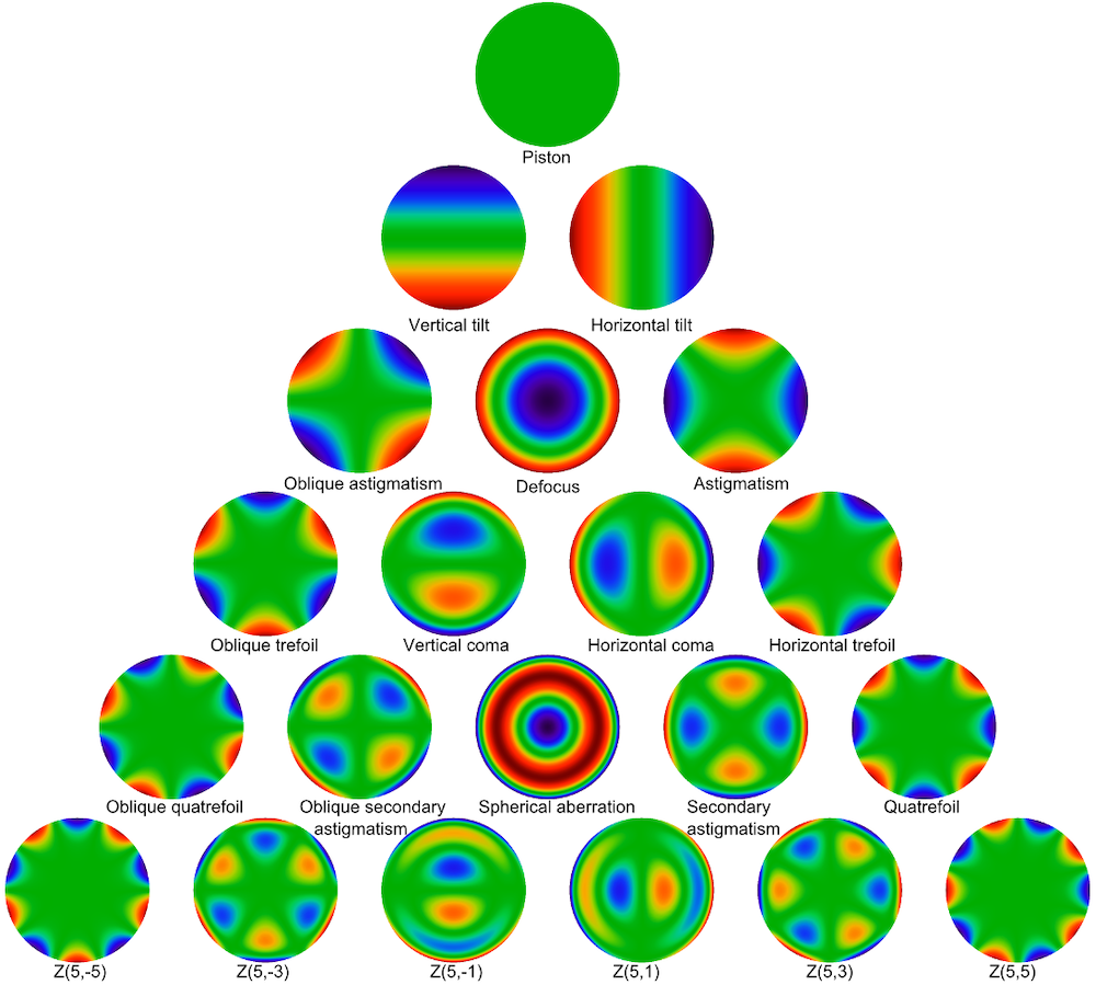
Plots of Zernike polynomials up to the fifth order.
Representing a Deformed Mirror with Zernike Polynomials
Finally, let us put our knowledge to use in an example problem. The geometry is a flat cylindrical mirror that is fixed on the sides and bottom, while the top surface may deform freely. The lens is uniformly heated, generating thermal stress and causing the top surface of the mirror to expand.

Geometry of the undeformed mirror (left) and deformed mirror (right).
We wish to compute the Zernike polynomial coefficients that will best fit the displacement field of the deformed surface of the mirror. As shown in the following screenshots, we will include all Zernike polynomials up to fourth order for the sake of completeness, although only the terms with a meridional index of 0 (the piston Z_0^0, defocus Z_2^0, and spherical aberration Z_4^0) play a significant role due to the symmetry of the displacement field. To integrate the product of the displacement with each Zernike polynomial, an Integration coupling is defined on the deformed surface. Some Variables nodes were then used to define the integral of the product of each Zernike polynomial with the solution vector, which determine the values of the corresponding Zernike coefficients.
Finally, we plot the out-of-plane component of the displacement field w on a cut line extending radially outward from the center of the mirror and compare it to the linear combination of Zernike polynomials. The following plot shows the individual combinations of the piston, defocus, and spherical aberration terms, and also compares their linear combination to the displacement field. The agreement between the solution and the Zernike polynomial fit looks quite good, and could be improved further by including higher-order terms, such as Z_6^0.
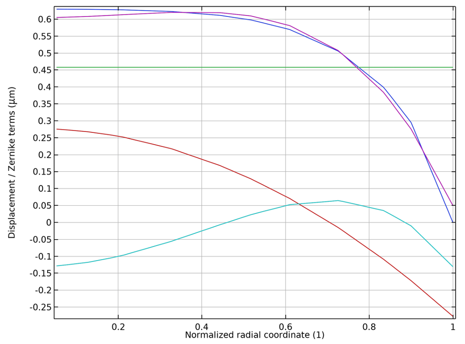
Comparison of the displacement field (blue) with the Zernike polynomial fit (purple). The piston (green), defocus (red), and spherical aberration (cyan) terms are also shown individually.
Conclusion
While curve fitting is an excellent tool for smoothing out statistical noise in experimental data, it also can be applied to the model solution itself, to great effect. Fitting the solution data to a set of predefined functions, especially orthogonal functions, offers a quick and convenient means of data compaction.
Next Step
Try out the model discussed in this blog post yourself by clicking the button below, which will take you to the Application Gallery entry and downloadable MPH-file.
References
- ISO 24157:2008: Ophthalmic optics and instruments — Reporting aberrations of the human eye, International Organization for Standardization, Geneva, Switzerland. Amendment 1, ibid., 2019.
- ANSI Z80.28-2017: American National Standard for Ophthalmics — Methods of Reporting Optical Aberrations of Eyes. American National Standards Institute, Alexandria, VA.


Comments (4)
Ivar KJELBERG
July 30, 2021Hi Christopher,
Thanks for a nice Blog, indeed the Zernike coefficients are very commonly used in optics (Bessel functions are also sometimes used as these are easier normalised), but Zernike also applies for structural analysis of i.e. the gravity (or boundary force load) deformations of large mirrors, for my case it’s mostly deformations of the M1, M2, … Mn of large telescope optics. Here mostly the light is assumed perpendicular to the nominal mirror surface and it’s generally sufficient to use the surface deformation as arguments for the Zernike polynomial analysis (with a factor 2 for the dual pass after the reflection on the mirror surface).
It would be really nice if we could use, in a more general way, your Zernike operators of the Optics Ray tracing module for all COMSOL modules (at least those related to “solid” and HT). So that we could use a consistent and similar operator for the Zernike analysis for both structural load deformation, as thermal, and full optics analysis.
We get the device specification of telescope mirrors with requirements on the Optical (or Mirror = 1/2) Wave Front deformations as Zernike coefficients to be assured, and this design work then falls back on both the designer of the mirror and the polisher, but also on the designer of the support structure of the large mirrors. And these mirrors of several metres diameter today are supported by active devices such to apply force loads at different points on the mirrors and then we must statically, and sometimes dynamically analyse the optical mirror surface deformations to sub micron levels such to show we meet the requirements. Today, I must rewrite my own Zernike analysis script each time, check and validate it, then apply it, while now you have one already in the Optical Ray tracing module, but as I understand it I must set up a full ray tracing analysis, while in fact it’s sufficient for the “mechanical” designer to deliver a Zernike analysis only applying to the mirror surface deformations (u,v,w) w.r.t. a given normal direction (nx,ny,nz). And I’m sure this is the case for many of us working in the Space, or Astro science development.
The exceptional thing with COMSOL is that we may now analyse not only the optical performance, but we may optimise the mechanical, the actuator (often ACDC or pneumatic devices) and even the control loop design all, in the same analysis tool: COMSOL Multiphysics(r) !
Including a full STOP analysis, the best dream for a System Designer 🙂
Sincerely
Ivar
Erik Hebestreit
July 30, 2021Hi Christopher,
I agree with Ivar, nice blog article. This topic is particularly useful for people in optics, where surface imperfections are often characterized with Zernike polynomials. Previously, I have done fitting using ODEs as explained in the article you mentioned (Curve Fitting of Experimental Data with COMSOL Multiphysics). While this approach is very versatile (you don’t need any orthogonal set of functions), unfortunately it quickly becomes very slow. Your approach is more elegant for this specific case and probably more efficient for bigger models. I’ll try it out on one of my models soon!
Best,
Erik
Christopher Boucher
August 5, 2021 COMSOL EmployeeHi Ivar, Erik, thanks for reading and commenting! I think that Ivar is referring not just to the built-in Zernike functions in COMSOL but also to the dedicated postprocessing features, the “Optical Aberration” plot and “Aberration Evaluation” node, for the Ray Optics Module, which take the optical path difference among rays and compute the corresponding Zernike coefficients. I agree in general that the capability of these features could be extended in a number of different ways.
Ivar KJELBERG
August 9, 2021Hello Christopher
indeed, I have a tendency to push for generalisations, and here I believe you might have the possibility to allow us to also use your optical ray tracing plots and postprocessing for not only optics variables, but also finally structural variables, as a structural deformation has units “meters” but OPD’s, when referred to wavelengths, too …