

Many different tools are available for counting particles. Choosing the optimal method depends on the application; specifically, whether you want to use the number of counted particles in equations or during postprocessing. The Particle Tracing interfaces in COMSOL Multiphysics feature three main particle counting options. While these approaches are versatile enough to compute quantities such as charge density and momentum flux, our focus here will be computing the number of particles on a set of domains or boundaries.
Three Particle Counting Approaches
During Postprocessing
When it comes to counting particles, the easiest way to do so is directly within postprocessing, after the solution has been computed. Let’s walk through the steps behind this basic methodology.
First, create a duplicate of the default Particle Data Set, which is automatically generated after computing the solution. Add a Selection to the data set, as illustrated below, and then select the domains or boundaries in which you will count the particles.

Next, add a Global Evaluation node under Derived Values and point to the new Particle Data Set, in this case, Particle 2. You can select specific parameter values or output times in the settings window.

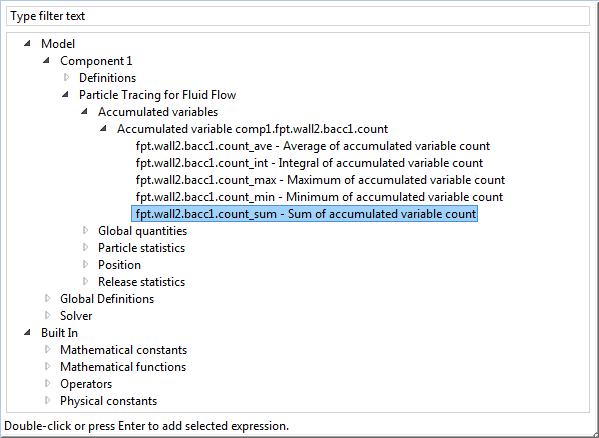
Choose from the following predefined expressions under the Particle statistics section in the Add/Replace Expression menu:
- <
phys>.alpha— Transmission probability (the number of particles in the selection specified by the Particle Data Set divided by the total number of particles). - <
phys>.Nsel— Total number of particles in selection (the number of particles in the selection specified by the Particle Data Set). - <
phys>.Nt— Total number of particles (the total number of particles in the entire model).
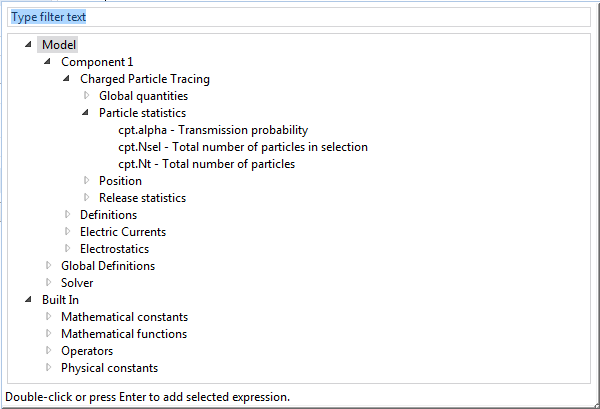
Evaluating the Global Evaluation node will display the value of the expression in a results table.
Application Library Examples
- Molecular Flow Module > Industrial Applications > charge exchange cell
- AC/DC Module > Particle Tracing > quadrupole mass filter
Using Accumulators
If the number of particles or the number density of particles needs to be used in another physics interface, the best option is to use an Accumulator. Accumulators transfer information from particles to the mesh elements in which they reside. They are available on both domains and boundaries and can be accessed from the context menu of any Particle Tracing interface. Upon adding an accumulator to a domain, the following settings are shown:
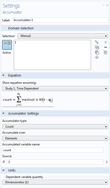
The available options in the Accumulator feature are:
- Accumulator type: When set to Count, the accumulated variable is simply counted in each mesh element, unaffected by the element size. For Density, the accumulated variable is divided by the volume of the mesh element, allowing you to compute quantities like the number density of particles.
- Accumulate over: When set to Elements, the accumulated variable is simply the sum of the source terms for all of the particles that reside in the element at a given point in time. When set to Elements and time, the particles leave behind a contribution in the elements that they pass through, based upon how long they were in each element.
- Source: This is the expression defined on the particle that you want to project onto the underlying mesh. When counting particles, Source is simply set to “1”, but it can be any expression that exists on the particles, such as charge or kinetic energy. It can also depend on variables that are defined in the domain in which the particles are located.
- Unit: When the unit is selected for the accumulated variable, the required unit for the Source will change accordingly.
To count the total number of particles, you can add an integration component coupling to the domain where the accumulator exists. Boundary accumulators automatically add component couplings on the selected boundaries. In our example, the total number of particles is then given by <integration_operator_name>(pt.count). This can be evaluated using the Global Evaluation node. The number of particles within each mesh element may also be coupled to other physics, since it is a degree of freedom. We can visualize how the particle counting works by plotting particle locations on a plot of the accumulated variable and the underlying mesh.
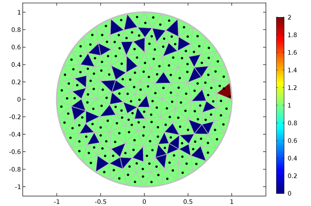
A plot shows the particle locations (black dots) on top of the underlying mesh (gray lines). The color in each element represents the value of the accumulated variable.
From the plot above, it is clear that the accumulator does indeed count the number of particles within each mesh element. For mesh elements in which there are no particles, the accumulated variable is zero, indicated by the mesh elements (shown in blue). Most mesh elements have one particle, which is highlighted in green. However, one mesh element happens to contain 2 particles (shown in red).
You can also use accumulators to count the number of particles passing through an interior boundary. To do this, simply add a Wall condition on the boundary that the particles will pass through, setting the Wall condition to Pass through. Add an Accumulator subfeature to the Wall node with the following settings:
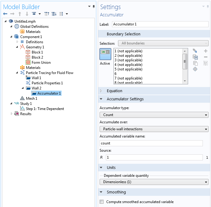
When a particle passes through the boundary, the accumulator increments the degree of freedom in the corresponding boundary mesh element. This gives the spatial distribution of the number of particles passing through the interior boundary, as depicted in the animation below.
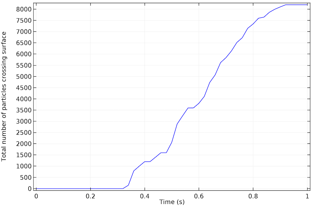
It is possible to conveniently plot the total number of particles passing through the boundary as a function of time. Simply add a 1D Plot Group and a Global plot feature. The accumulator creates predefined variables to add up the accumulated variables over all the mesh elements. To get the total number of particles, you can use the Sum of accumulated variable count option.
The plot below shows the results for the total number of particles that crossed the interior boundary.
Note: To learn more about the applications of accumulators, you can refer to this earlier blog post by my colleague Christopher Boucher.
Application Library Examples
- Molecular Flow Module > Benchmarks > s_bend_benchmark
Particle Counter, New in COMSOL Multiphysics Version 5.2
A Particle Counter is a domain or boundary feature that provides information about particles arriving on a set of selected domains or surfaces from a specified release feature. Such quantities include transmission probability, current, and mass flow rate. The settings for a Particle Counter feature are very simple. Select a Release feature to connect to, or select All release features. You can add Particle Counter features to the model and access their variables without having to recompute the solution. Simply use Study > Update Solution, and the new variables will be automatically generated and immediately available for evaluation.

Each Particle Counter generates the following expressions. Note that the scope is different than the variables that are always available in the Particle statistics plot group, as outlined in the first section.
- <
phys>.<feature>.rL— Logical expression for particle inclusion; can be used in the Filter node of the Particle Trajectories plot, allowing visualization of only the particles that connect a source and a destination. - <
phys>.<feature>.Nsel— Total number of particles in selection; computes the total number of particles released by a specific release feature in the set of domains or boundaries determined by the Particle Counter selection. - <
phys>.<feature>.Nfin,— The number of transmitted particles at the final time (the number of particles in the Particle Counter selection at the final solution time). - <
phys>.<feature>.alpha— Transmission probability (the ratio of the number of particles in the Particle Counter selection divided by the number of particles released by the release feature).
When the Release feature is a Particle Beam feature — a specialized release feature for the Charged Particle Tracing interface — additional variables for the average beam position, velocity, and kinetic energy are generated for the particles that connect the counter to the particle beam.
Application Library Examples
- Particle Tracing Module > Charged Particle Tracing > sensitive high resolution ion microprobe
- Particle Tracing Module > Tutorials > brownian motion
- Particle Tracing Module > Fluid Flow > laminar mixer particle
Summary of Counting Particles in COMSOL Multiphysics
There are three ways to count the number of particles on domains and boundaries. For simple models in which only a single release feature is present, the postprocessing tools might suffice. If you want to plot the number of particles on a domain or boundary, or if you want to use the number of particles in another physics interface, accumulators are the answer. To count particles that only connect a specific release feature to a selection of domains or boundaries, you can use the Particle Counter feature — one of the many new additions in COMSOL Multiphysics version 5.2.
Additional Resources
Access the MPH files and documentation for the tutorial models and demo application featured in this blog post at the links below.


Comments (10)
Sepideh Ramezani
November 23, 2015Hi Daniel,
Many thanks for useful blog post. I chose the first approach and I found strange result.
In selection if I choose “Entire geometry” which means the whole domain [Am I right?] entire geometry photo, then the number of particles are different from the one that I choose domain and the whole domain .
Is there any reason for this result?
More detail about my particle tracing module in my model: I released 100 particles and it seems that if I choose in selection “Entire Geometry” then this evaluation is not working correctly in COMSOL!
Hope to hear from you.
Sepideh
Signe Engelsholm
May 8, 2016Hi Daniel
IThank you for a nice post, it was very informative!
However, I would like to know hov you managed to make those plots of accumulated variables. When I plot it, I the values are evaluated in the nodes and not in the elements, so the plot looks quite different. It seems to me that what the accumulator really does is not exactly what you have explained here?
In addition I am very surprised to see that the _sum (sum of accumulated variable Count) is not identical to intop(), when the integration operator is set to “summation over nodes”.
Hope you can enlighten me 🙂
Signe
Tuan-Anh Le
October 21, 2016When I count particle by selection section, sum of its not equal release particle number. I don’t know why, plz help me to solve it
LEE
May 8, 2018Hi Daniel,
As you mentioned above, the “Accumulator” is available on both domains and boundaries. I am using COMSOL v5.3a, which can only select “Domains” in “Accumulator.” Is it a bug? Thanks.
Daniel Smith
May 9, 2018 COMSOL EmployeeHi How-Ming Lee, Accumulators can be added on boundaries by right clicking on the Wall node and selecting Accumulator.
Dan
Anonymous
July 5, 2018Hi Daniel,
Thank you for this good Presentation it was a really interesting topic and I am stuck on how to learn about to The total number of Particles crossing surface graph if you could recommend me an example treating this part.
I would really appreciate your help.
Imène Oualid.
waheed ul hassan
November 15, 2018Hi Daniel
(A plot shows the particle locations (black dots) on top of the underlying mesh (gray lines). The color in each element represents the value of the accumulated variable.) have you any example file for this type. Because i cannot understand exact method.
I would really appreciate your help.
Waheed
Kritik Saxena
February 28, 2021I am able to put the accumulator condition in the particle tracing part. But I could not understand how to see the results of that accumulator in animation form. Can someone please help me how to reach to animation stage below the text as follows: “When a particle passes through the boundary, the accumulator increments the degree of freedom in the corresponding boundary mesh element. This gives the spatial distribution of the number of particles passing through the interior boundary, as depicted in the animation below.”
Christopher Boucher
April 26, 2021 COMSOL EmployeeHi All,
We have received a number of questions about how to reproduce some images shown in this blog post, that include both the particle positions (as points) and a surface plot of the accumulated variable.
To recreate these images, add two plots to the same Plot Group: one “Particle Trajectories” plot and one “Surface” plot. The “Dataset” for each of the two plots should be “From parent”, and the dataset of the containing plot group should be a “Particle” dataset. There are other ways to make a similar image, but the advantage of having both plots point to the same dataset is that you can make animations much more easily.
For questions about a specific model, please do not hesitate to contact COMSOL support.
Kind Regards,
Chris Boucher
Adriel Wong
May 11, 2024Hi, I am simulating a microfluidic spiral channel. I have used the particle tracing feature and inputting 3 types of cells; Circulating Tumor Cells (CTC), Red Blood Cells (RBC) and White Blood Cells (RBC) according to their own particular size and density. CTC – 15 um – 1077 kg/m3 WBC – 10 um – 1080 kg/m3 RBC – 6 um – 1110 kg/m3
The results are well, showing the particle separating and eventually CTCs are separated from the RBCs and WBCs. Majority of CTCs ending up in outlet 1 while RBCs and WBCs end up in outlet 2. However, is there a proper way for me to tabulate a graph showing the types of cells and number of cells at the outlet? I do not want to tabulate the graph showing total number of cells as I want to distinguish between the number of CTCs, RBCs and WBCs at both outlets.
I have reviewed this blog: https://www.comsol.com/blogs/different-ways-to-count-particles-in-comsol-multiphysics/ But it shows methods to count total number of particles and not specifying the different particles.