Sometimes a simulation runs longer than needed, not giving us a way to monitor intermediate results or stop conditionally. This can leave us staring at the monitor, ready to pounce. In this blog post, we discuss how to automate this process in the COMSOL Multiphysics® software. This way, we can work on something else while the software checks the conditions after each step. We also have the option to see what happens the first time the conditions are violated.
Stop Conditions: When and How to Use Them
We often want to stop a time-dependent or parametric solver when a certain condition is met or violated. But we usually do not know the exact time or parameter value at which the stop condition is going to occur. In this case, we need to specify a solution time or parameter range large enough so that we are reasonably certain that the stop condition is going to be activated. We then add a stop condition to terminate the solver.
Physical conditions or computational issues can trigger a stop. Examples of such physical conditions include allowable stresses, temperature limits, and species depletion in reactions. As for computational issues, one example is a very small time step size taken by the solver.
In COMSOL Multiphysics, a stop condition can be added to the following solvers:
- Time-dependent solver
- Frequency-domain solver
- Stationary solver with a parametric or auxiliary sweep
The first step is to define a scalar that we can use in a relational or logical expression. This scalar can either be a quantity defined at some point of interest or a global quantity, such as an integral, maximum value, minimum value, or average of a variable over domains or boundaries. In the software, we can define this using a point probe or a component coupling. The second step is adding a stop condition to the solver configuration. The condition has to be a statement that evaluates to true or false.
Using Stop Conditions in Time-Dependent Solvers
To demonstrate how to set up a stop condition, let’s look at a time-dependent heat transfer problem. We will tell the software to stop the computation when the maximum temperature exceeds a threshold value. (We can also use different conditions, but the procedure remains the same.)
Consider a silicon wafer heated by a moving heat pulse and cooled via radiation to the surroundings. (For more details, check out the tutorial model.) In this case, we want to modify the model such that the computation stops when a threshold temperature is reached.
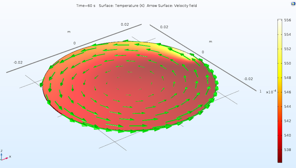
The temperature distribution on a rotating wafer heated by a moving heat pulse.
To start, we define a scalar by using integrals, averages, maxima, or minima evaluated over geometric entities. If we are interested in what happens at a specific point, a point probe or an integration component coupling can be used. In this example, the scalar that we monitor is the maximum temperature. This can be obtained using the Maximum component coupling.
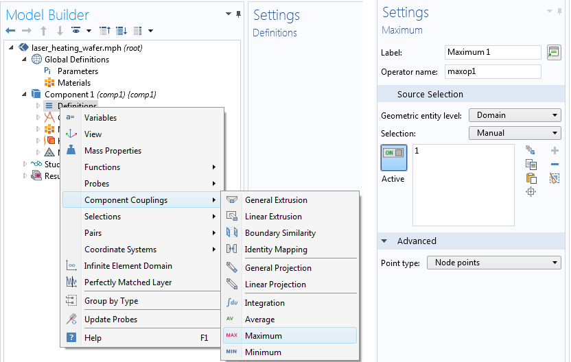
Steps for adding the Maximum component coupling.
When we compute the study for the first time, we use the Show Default Solver command to open the settings. Then, we can go to the Time-Dependent Solver node under Solver Configurations and add a Stop Condition node.

A Stop Condition node can be added to the Time-Dependent Solver node in the solver configurations.
The final step is to add the expression and conditions in the Stop Condition Settings window.
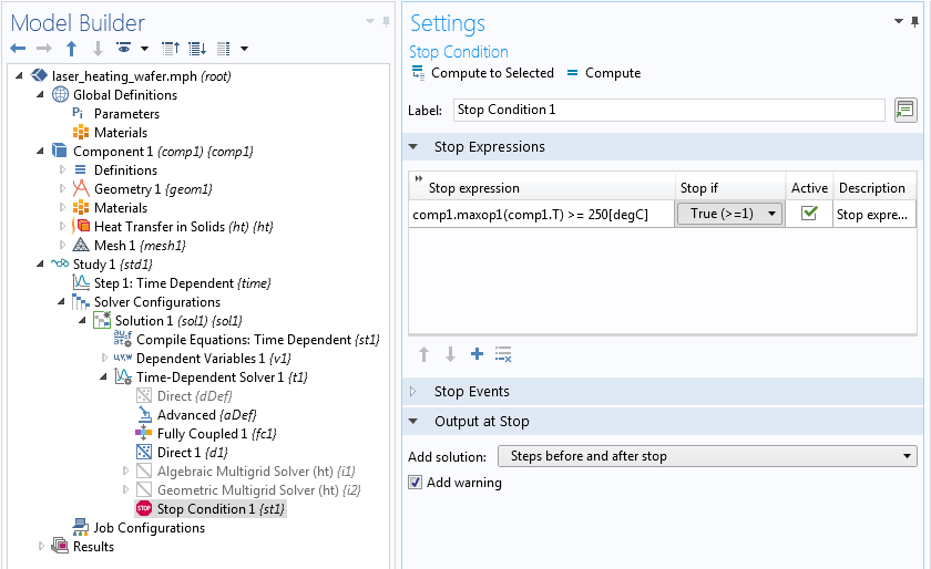
The Stop Condition Settings window for a time-dependent solver.
The stop condition above stops the solver when the maximum temperature is greater than or equal to 250°C.
The solver stops after 27.238 seconds because the stop condition has been satisfied (even though we asked it to compute up to 60 seconds in the study settings). We can see the cutoff time in the Warnings node that the solver adds in the solver sequence.

By default, the solver adds a Warnings node if the computation is terminated by a stop condition.
In the Stop Condition Settings window, we use the comp1 name scope to identify both the maximum operator and the temperature variable T. These are items defined under Component 1, whereas the solver sequence is a global item. For example, if we have a second component in our model and redefine maxop1 there, the solver sequence cannot tell which operator we are referring to. Thus, we must use the component identifier.
Note that we can choose whether or not we want to stop when the condition is true or false. Additionally, in the Output at Stop section, we can decide if we want to add a time step just before or after the stop condition is met.
If we have an Event interface in the Model Builder, we can use it as a stop condition by adding it under Stop Events in the Stop Condition Settings window.
Stopping When Time Steps Are Too Small
The time-dependent solvers in COMSOL Multiphysics are adaptive. As such, the time steps are picked based on user-specified error tolerances and computed local error estimates. When the error estimates are very high, the software takes smaller and smaller steps. For example, this happens when the solution becomes singular. If we want to stop the solver when the time steps are too small, rather than trying to approach this singularity with increasingly smaller and smaller time steps, we can add a stop condition based on the reserved variable timestep.
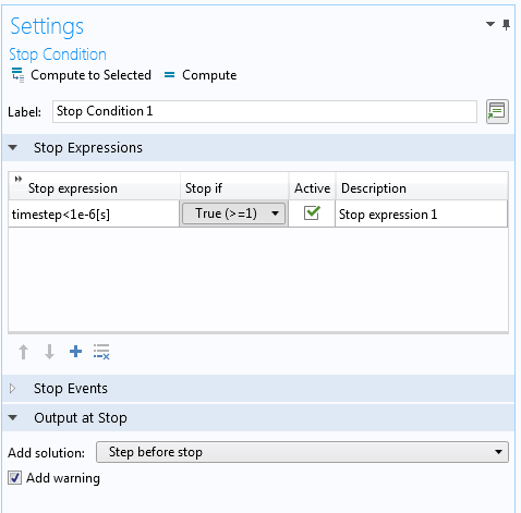
Since timestep is a predefined global parameter, it is recognized without a name scope.
Stop Conditions in Parametric Solvers
Stop conditions can be added to frequency-domain studies as well as parameterized stationary studies. Parameterized stationary studies can either be regular parametric sweeps or auxiliary sweeps. In all of these cases, the Stop Condition node should be added to the Parametric node under Solver Configurations > Stationary Solver.
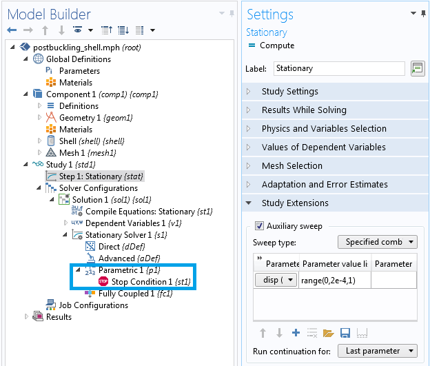
Stop conditions can be added in stationary analyses when performing an auxiliary or parametric sweep.
Note that, as in the time-dependent problem, we need a scalar variable to monitor and must use the right variable scope in the stop condition.
To see how to use a stop condition in an auxiliary sweep to implement a nonstandard load ramping procedure, check out the example model of a postbuckling analysis of a shell structure.
Variable, Function, and Component Coupling Namespaces
Expressions used in the stop condition and other items in the solver configuration have to be global to be automatically recognized. Otherwise, we have to provide the component name as a prefix. This is the case for every variable (including physics variables like T for temperature) and functions inside a component. On the other hand, parameters defined under Global Definitions in the Model Builder are recognized without the component prefix.
For example, when referring to the built-in integration operator, we can simply use integrate. In contrast, when referring to the integration operator myint that is defined in component comp1, we have to use comp1.myint.
The following predefined constants, variables, functions, and operators can be used in the solver configuration without identifying a component:
- Physical constants, such as the gravitational acceleration g_const
- Mathematical constants, such as pi
- Built-in global variables, such as t for time and freq for frequency
- Built-in mathematical functions, such as trigonometric and exponential functions
- Built-in operators, such as differentiation and integration operators
See the COMSOL Reference Manual for a full list and syntax.
In this blog post, we have discussed how to add conditions that stop a time-dependent or parametric solver when one or more criterion is met. If you have any questions related to this topic or using COMSOL Multiphysics, contact us via the button below.
Related Resources
- Learn about other ways you can improve your modeling process:


Comments (2)
Jesus Lucio
August 2, 2021Hi Temesgen,
Thanks a lot for this blog. It’s very helpful.
But what about continuing the simulation after the stop condition in a time dependent study? In particular, if the stop condition interrupts the solution in (time dependent) step 1 and we have another time dependent step (step 2) after it, how can we express in step 2 the latest time given in step 1 before computing the solution? The simple “t”, as in “range(t,0.01,6)” does not work, but even “withsol(‘sol1’,t)” does not succeed.
Regards,
Jesus.
Sagar Rao
June 6, 2023Hi Jesus,
It is of course a late response (and I am not responding on behalf of COMSOL, just as a user), but perhaps this could be useful to anyone else who comes here as well – I tried this out with COMSOL 6.1 and it seems to work.
Once the study steps are defined, one would look into the solver sequence and insert a “Stop” condition as explained in the article already to the Solver node linked to the relevant study step (e.g. Study 1 -> Solver Configurations -> Solution 1 -> Time-Dependent Solver 1 -> insert a stop condition). At this point, if the results of the corresponding study step are to be automatically transferred to a subsequent step as the start condition, it is as straightforward as
1) Opening the study step that should receive the result,
2) Navigating to “Values of Dependent Variables”,
3) Set “Initial values of variables solved for” to “User Controlled”,
4) Pick the “Solution” option under “Method”,
5) Under “Study”, select the study step which was stopped by the “Stop” condition,l
6) Select the relevant solution, and
7) for “Time (s)”, use “Last”.
This should immediately redirect the receiving solver step to begin from the stopped condition, since that is the “Last” solution stored by the previous study step.
Do let me know if there is any confusion in the steps above, or if it is not written clearly enough.