The Hall effect sensor is commonly used for position sensing. The basic working principle is that a nearby magnetic field deflects the path of current through a semiconductive sensor. This deflection of current causes a change in potential, which can be measured. Despite the multiphysics nature of this device, with a couple of assumptions, it’s actually possible to model it very simply in the COMSOL Multiphysics® software. Keep reading to find out more…
Basic Working Principle of a Hall Effect Sensor
We will start with the definition of the Lorentz force, the expression for the total force on a charged particle moving through an electric field, \mathbf{E}, and a magnetic field, \mathbf{B}, at a velocity, \mathbf{v}. The total force on a particle, of charge q, is:
Let’s consider a slab of semiconductive material with an electric potential difference applied across two ends that causes current to flow. For a uniform slab, the current will flow in a straight line between the two terminals. However, due to the Lorentz force, any nearby magnetic field will deflect this current path, thus altering the electric potential distribution within the material, and this can be measured. For typical Hall effect sensors, the magnetic field is due to a nearby magnet.
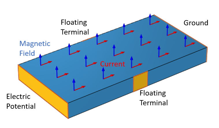
A slab of semiconductive material. Current passing through the material will be deflected by the magnetic field, which will change the electric potential between the two floating terminals.
In terms of the equations that we will use within our computational model, we start with the above equation and write the current density through the semiconductive material as a function of the electric field and the magnetic field, as well as two additional material constants, the electric conductivity, \sigma, and R_H, the Hall coefficient:
We can rewrite the above as a matrix-vector multiplication:
That is, the Hall effect can be modeled simply by defining an anisotropic electric conductivity that is a function of the magnetic field. For brevity, we will omit discussion of sign conventions and the derivation of the Hall coefficient in different materials. This is the unique constitutive relation that we need to incorporate into our computational model.
Now, in the simplest situation, we could just assume a given magnetic field, and use that to compute the electric conductivity, but what we will do here is compute the varying magnetic field and use that to create a true multiphysics model.
Before we start any modeling, though, we will make a few assumptions to simplify things. We will assume that the time rate of change in the magnetic field is sufficiently slow enough that it can be ignored. That is, although the Maxwell–Faraday equation states that:
we will assume that \frac{\partial \mathbf{B} }{\partial t} is negligible and can be ignored.
This is equivalent to saying that there are no significant induced eddy currents in the semiconductive slab due to the motion of the magnet. That is, the electric field in the material is due solely to the applied electric potential and aforementioned constitutive relationship, and not directly due to any time variation of the magnetic field. This assumption lets us reduce the problem to solving for the magnetostatic fields.
Next, we will also assume that the currents flowing through the semiconductor are small enough that they do not themselves produce any significant magnetic field as compared to the magnetic field due to the magnet. This reduces the magnetostatic problem to the so-called current-free form, wherein we only need to solve for a magnetic scalar potential. Note, however, that these assumptions are not necessary for what we’re about to do. We could also solve for the magnetic fields due to currents, such as from a nearby coil. This would only make our model a bit more computationally expensive.
Lastly, we will also assume that the conductivity of the material is large enough such that the RC time constant is much shorter than any time variation that we are interested in. That is, we can, at any instant in time, treat the electric currents model as a purely static situation, since we’ve assumed that all time derivative terms are unimportant. So, the electric problem reduces to solving for the stationary electric potential equation, albeit with a spatially varying anisotropic electric conductivity that is a function of the magnetic field.
With all that said, we are ready to begin our modeling!
Implementing the Model in COMSOL Multiphysics®
We will consider the situation in the image below. A small cylindrical magnet is mounted on a rotating iron wheel. Below, there is a rectangular domain representing the sensor.
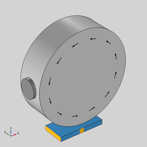
Schematic of a Hall effect sensor placed underneath a rotating iron wheel with a magnet mounted on the rim.
We will solve first for the magnetic fields, using the Magnetic Fields, No Currents interface. In addition to the domains pictured above, we model the air space surrounding these, as well as an Infinite Element truncation domain.
Solving this problem, we compute the magnetic fields, and can then move on to the model of the Hall effect sensor. In the semiconductor domain, we use the Electric Currents interface. The Ground and Terminal conditions are applied at opposite ends of the material, and two Floating Potential conditions are applied on either side.
For a quick introduction to the usage of the Electric Currents interface, see our series of tutorial videos on resistive device modeling.
The electric conductivity can be made a function of the spatially varying magnetic field, which we just computed, but we would also like to consider the rotation of the wheel. The simplest way of considering rotation is to perform a Parametric Sweep, but that is actually a bit more than we need to do here. The magnetic fields are rotating through the sensor, but we assumed that they are unaffected by the sensor itself.
In this situation, we can just use a rotational mapping to change the magnetic field as a function of a global parameter, Angle, via the General Extrusion operator, similar to as described in this previous blog post. In this case, though, we’re rotating a vector field, so we also rotate the vectors themselves, via a 3D rotation matrix. The two screenshots below show the implementation and define a set of rotated magnetic field variables.
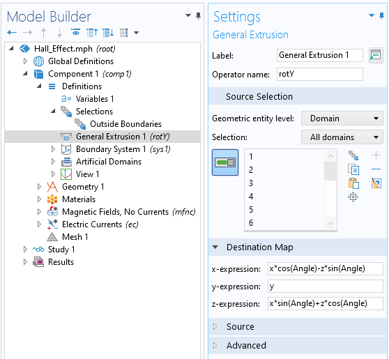
The General Extrusion operator defines a rotation about the y-axis.
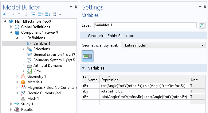
The variables defining the rotated magnetic field components.
Once we have these rotated magnetic field components, we can use them to define the electric conductivity tensor within the Electric Currents interface, as shown in the screenshot below.
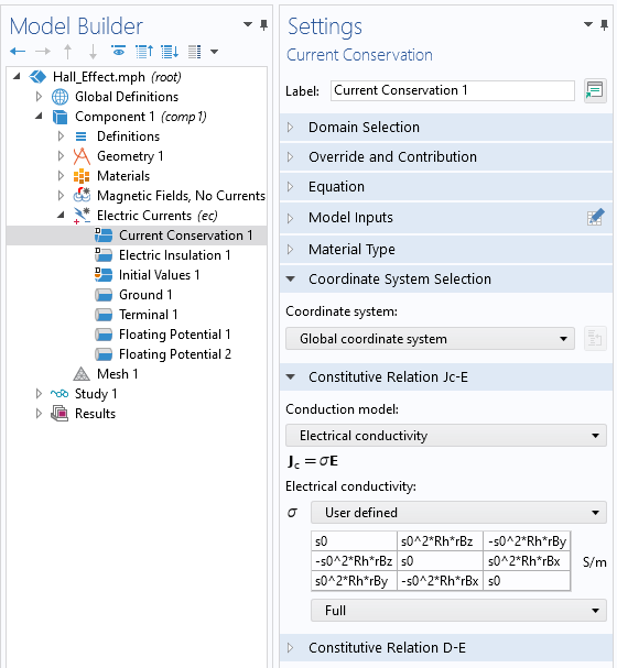
Defining the anisotropic electric conductivity within the Hall effect sensor.
With that, we are ready to solve the model. We can solve in two steps, first solving for the steady-state magnetic field, and then solving for the steady-state current, but with the magnetic field rotated through different angles via an auxiliary sweep, as shown in the screenshot below.
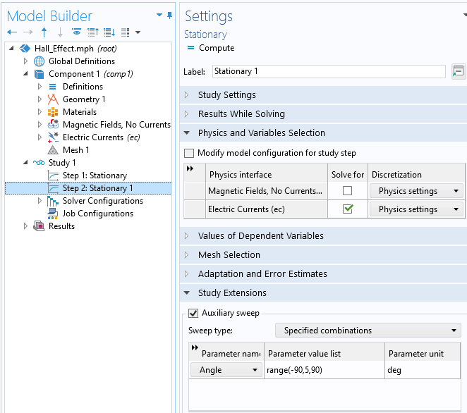
Setup of the solver. The magnetic fields are computed in the first step, and in the second step, the electric potential in the sensor is computed for different rotation angles of the magnet.
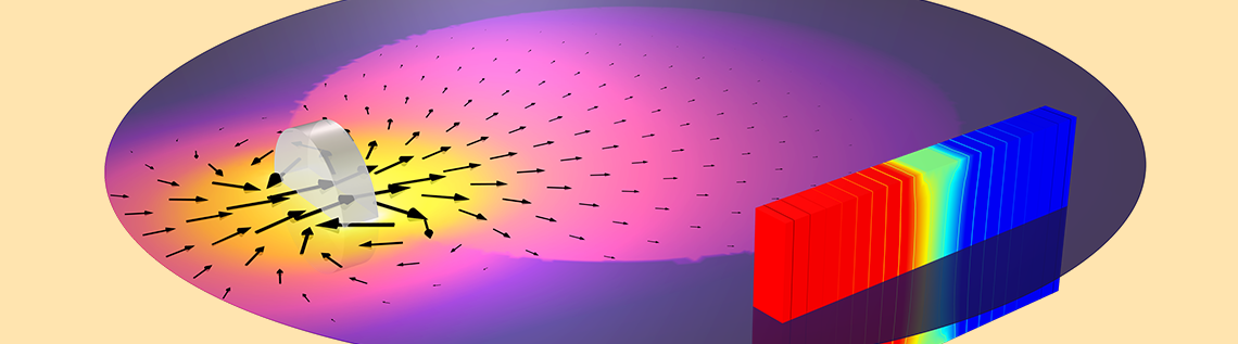
After solving, we can animate the rotating fields, to confirm our approach, and examine a plot of the difference in the electric potential between the two floating potential boundary conditions on either side of the sensor.
Animation of the rotation of the magnet and the magnetic field through the Hall effect sensor.
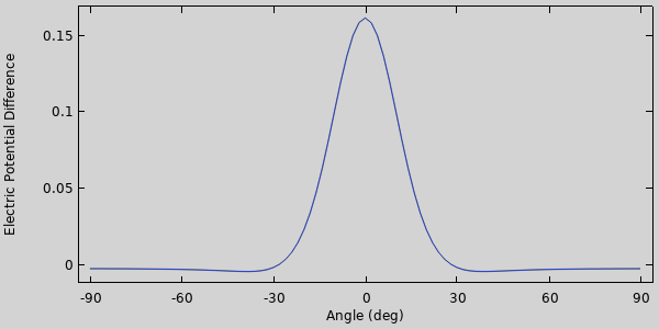
Variation in the electric potential between the two floating potentials on the sensor with respect to angle.
Try It Yourself
We’ve shown a simple way of modeling a Hall effect sensor. The ability to enter an anisotropic electric conductivity that is a function of any other variable in the model makes this kind of simulation very easy. By manually rotating the fields via a set of transforms, we can also greatly reduce the computational cost. The model is available for download via the link below.


Comments (7)
Harshitha Govindaraju
September 13, 2022Hello,
Thank you for the post. Now, how do we model a magnet moving along the x-axis of the semiconductor and not the rotational. What is the role of the rotational iron wheel?
Walter Frei
September 13, 2022 COMSOL EmployeeLinear motion can be modeled in a similar fashion as the rotational motion, via the Extrusion Operators, the expression would simply vary linearly along one axis. The iron wheel here is for demonstration purposes.
Harshitha Govindaraju
July 21, 2023Hi, thank you for the response. Which model has been used for the Hall field here? Ideally, the hall field meets the relationship: E= JX(B*RH). Please let me know.
Thank you again!
Walter Frei
July 24, 2023 COMSOL EmployeeThe Hall effect current is now part of the Electric Currents interface, see the documentation here:
https://doc.comsol.com/6.1/docserver/#!/com.comsol.help.acdc/acdc_ug_electric_fields.07.048.html
Prasanna Kumar Routray
February 21, 2024Hi Walter,
Thanks for your valuable contribution.
You use “Electric Currents” and “Magnetic Fields, No Currents” in this example. I want to use an electromagnet and Hall effect sensing mechanism, so I choose “Magnetic Fields” instead of “Magnetic Fields, No Currents”. Do you have any working example where both electromagnet and permanent magnet field can be sensed using a Hall sensing mechanism?
Thanks.
Prasanna Kumar Routray
February 21, 2024Hi Walter,
I’m trying to use “Magnetic Fields” instead of Magnetic Fields, No Currents to use an electromagnet, and still read the Hall Sensor response.
Still figuring out how to get it done.
Daiyan Ibnul Aswad
April 6, 2026Hello. I want to know that for a three phase Low Voltage distribution power system, in order to detect faults, how am I going to model the hall sensor in COMSOL?