
I watched the latest Top Gun movie, Top Gun: Maverick, a few weeks ago. It is a really awesome movie, and it is also cutting edge from an engineering standpoint. The movie starts with Maverick, played by Tom Cruise, working as a test pilot preparing to fly a new secretly developed airplane, the Darkstar, capable of flying Mach 10. Simultaneously, Rear Admiral Chester Cain, played by Ed Harris, makes his way to the test base to shut down the program — considering the Darkstar had not yet been able to fly Mach 10, which was a requirement for the project to continue — but Maverick takes action before Cain can do so. Just as Cain arrives to the base, Maverick takes off with the Darkstar to make a try for Mach 10. A great start!
The Shock Waves
At 9 minutes and 47 seconds into Top Gun, admiral Cain is sitting in the control room together with the Darkstar team looking at the mission control screens when the camera zooms in on one particular screen in the control room. It shows the density gradients around the airplane, visualizing the shock waves in a so-called schlieren image. After replaying this scene several times, I questioned how they could portray these visuals without the presence of a follower jet flying near the Darkstar using an air-to-air schlieren technique to visualize the shock wave pattern. No jet would be able to follow to record this? However, it occurred to me that they were using a digital twin that was live updating the simulation as Maverick maneuvered the airplane closer to the limit of Mach 10. At that moment, I also noticed that the speed shown on the control room display did not match the shock waves: the angle was too high. The angle depicted between the shock wave and the Darkstar’s fuselage appeared closer to Mach 1.1–1.2 rather than the actual Mach 7.5–8 speed during that time; this must have been a goof.
There came the inspiration for this blog post: What would the true shock waves and velocity field look like around the Darkstar at that speed? I decided to make a model and see what fiction left out. (In reality, such a model could be used to train a surrogate model for a digital twin, such as the one displayed in the control room.)
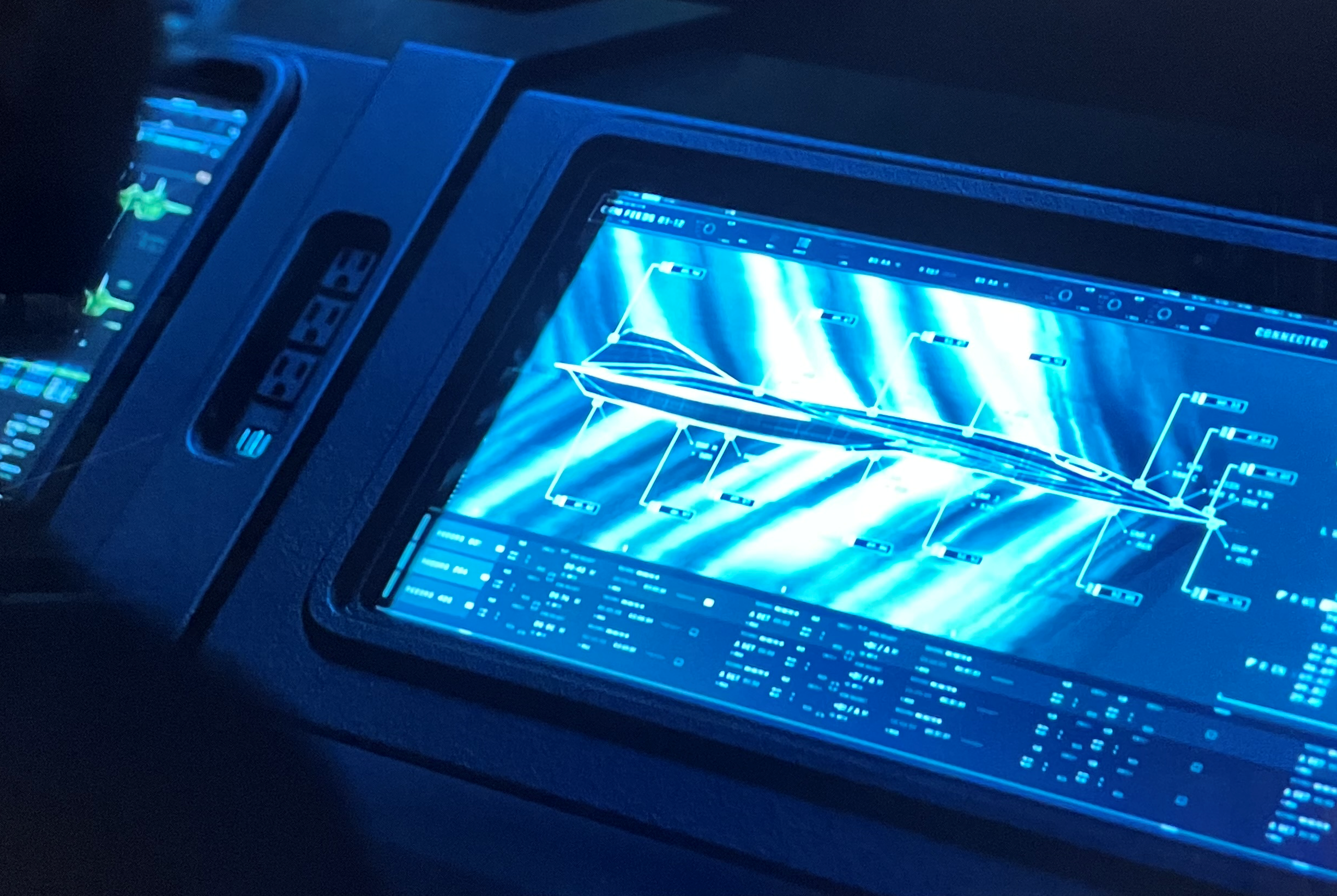
Figure 1. The digital twin of the Darkstar showing the shock wave pattern on the screen in the control room.
Modeling the Darkstar’s Geometry
Creating the model geometry could have been done relatively easily by purchasing physical 3D models of the Darkstar, such as 3D printed models, or CAD files. However, I chose to start from scratch and enlisted the assistance from the CAD team to help complete the task. Due to the limited project timeframe and challenges in obtaining accurate details, we omitted some details in the final geometry. We primarily relied on movie images and a few images of the real Darkstar prototype featured in the film.
The model geometry can be seen in the figure below. Note that in the second side-view image, you can see the compartment for the combined cycle propulsion, with a closed turbine inlet and an open scramjet inlet.
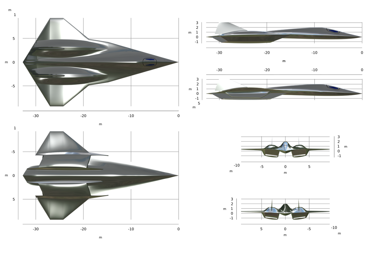
Figure 2. The Darkstar geometry.
Determining the Speed
In our first model, shown in Figure 3, the Darkstar is flying at a speed of Mach 1.5. We used an inviscid flow model as an initial approach to visualizing the shock pattern around the Darkstar’s fuselage. Figure 3 also shows the magnitude of the gradient of air density plotted on a horizontal plane together with the velocity field streamlines. The density gradients are revealed by the schlieren images in the real world.
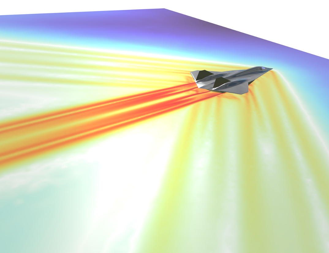

Figure 3. The Darkstar flying at a speed of Mach 1.5. The results show the density gradients caused by the shock waves and velocity streamlines.
Figure 4 shows a vertical and a horizontal slice cutting through the middle of the Darkstar along the length of the fuselage. The vertical plane figure corresponds to the schlieren image shown in the control room display in the movie.
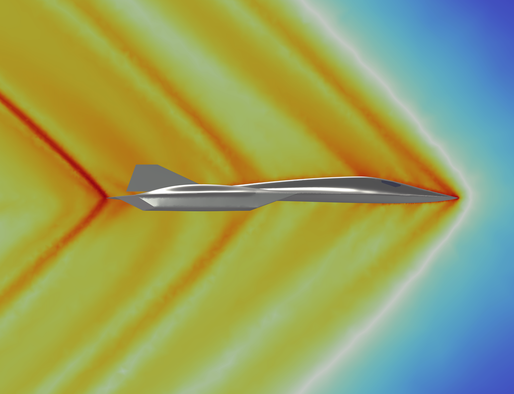
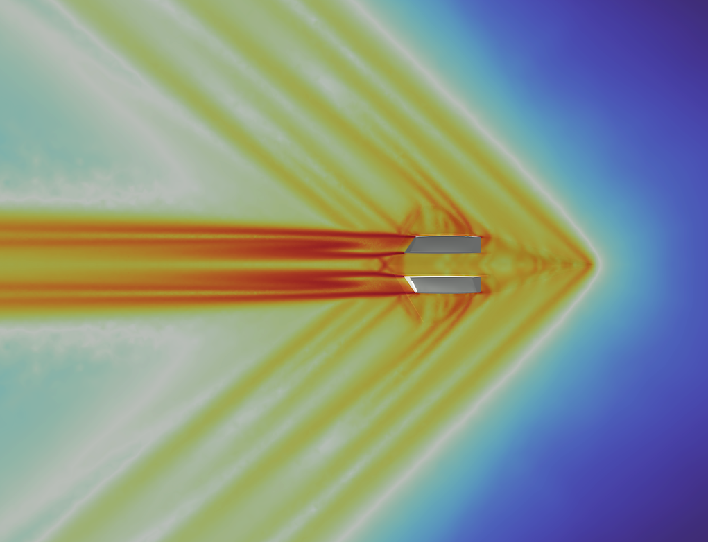
Figure 4. Magnitude of the gradient of density from the side (left) and from below (right) at Mach 1.5.
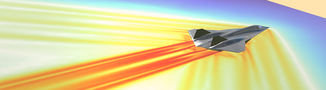
As mentioned, 9 minutes and 47 seconds into the movie, the Darkstar is flying at about Mach 7.5. In Figure 5, we see the shock waves from the side (left) and from below (right) at Mach 7.5. Note that we are plotting the logarithm of the gradient of the density. The white ripples in front of the Darkstar are noise caused by the numerical stabilization and are of the order of magnitude 1·10-7 kg/m3 or less.
The schlieren image for Mach 7.5 looks almost horizontal, which is different from what the digital twin shows in the control room in the movie. We will assume that this was intentional; the Skunk Works engineers who developed the Darkstar for the movie likely saw that the speed was a lot lower than Mach 7.5 but were satisfied with the visuals it produced.
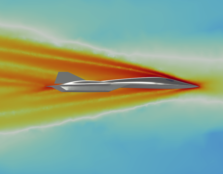
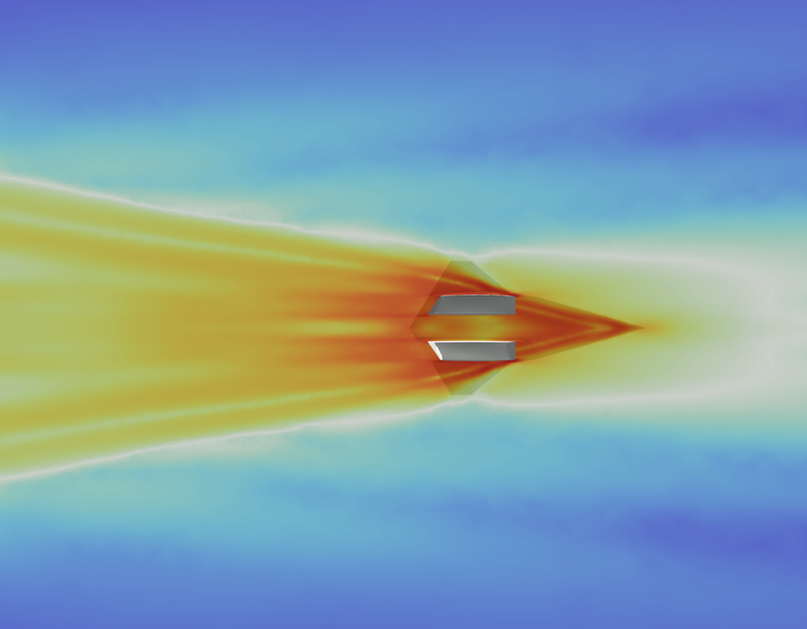
Figure 5. Magnitude of the density gradient of density from the side (left) and from below (right) at Mach 7.5.
The isosurfaces of the Mach number are shown in Figure 6. The left image shows the Darkstar flying at Mach 1.5, while the right image shows it flying at Mach 7.5. Since the isosurfaces are computed directly from the speed and not from the gradient of a field, they are smoother than the density gradients shown in Figure 5. The isosurfaces are plotted on half of the geometry, with a vertical symmetry plane cutting through the middle of the Darkstar along the length of the fuselage.
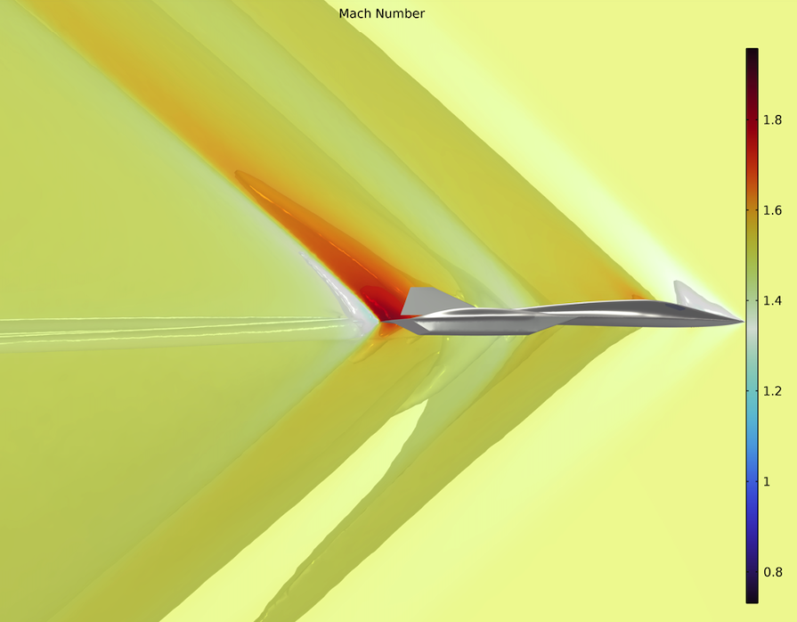
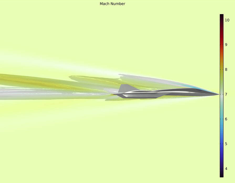
Figure 6. Plotted airflow, with the Darkstar flying at Mach 1.5 (left) and Mach 7.5 (right).
In the CFD simulations shown above, we used the High Mach Number Flow interface in the COMSOL Multiphysics® software. This physics interface solves for conservation of energy, mass, and momentum.
After creating the geometry and simulating the high Mach number flow, I thought to myself why limit ourselves to only that when we could further explore the stealthiness of the Darkstar…
How Stealthy Is the Darkstar?
The Darkstar is a large aircraft, as large as the legendary SR-71 Blackbird and twice as long as the F-35 Lightning II. Based on the high Mach number flow models discussed above, we have concluded that you can hear the Darkstar. However, we have yet to determine how visible it is to a radar and how large its radar cross section is.
The Darkstar would be flying at such a high speed that it would be difficult for enemy missiles to catch up (it would outfly most of today’s weapons). Yet, it’s interesting to know how the Darkstar compares to other jets when it comes to early detection. Early detection radars use frequencies between 1 GHz (wavelength = 30 cm) and 3 GHz (wavelength = 10 cm), which correspond to the L-band and the S-band, respectively.
Figure 7 shows the surface currents on the Darkstar’s fuselage from a vertically polarized frontal radar wave, incoming from the opposite flight direction. We can see that the reflections from the radome and the engine cover are pronounced at both 1 GHz and 3 GHz. However, the reflections from the vertical stabilizers are much more pronounced at 1 GHz compared to 3 GHz. In addition, the reflection at 3 GHz appear softer, resembling the effect of illuminating the airplane with a directional light from the front. This outcome is to be expected, as the higher the frequency, the closer we get to the physical optics approximation.
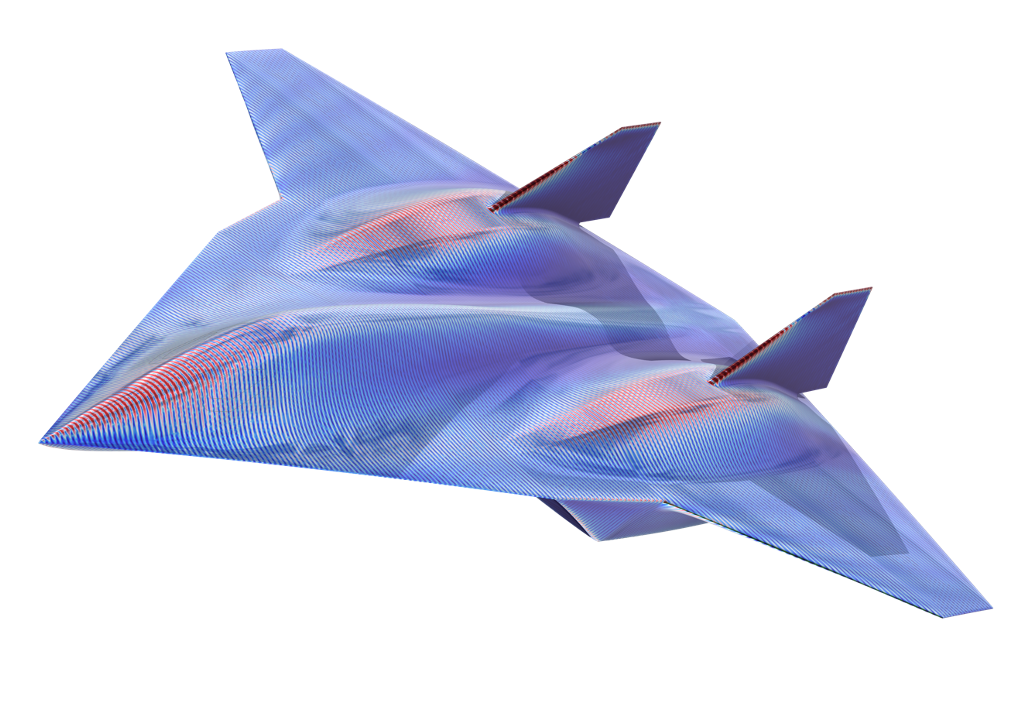
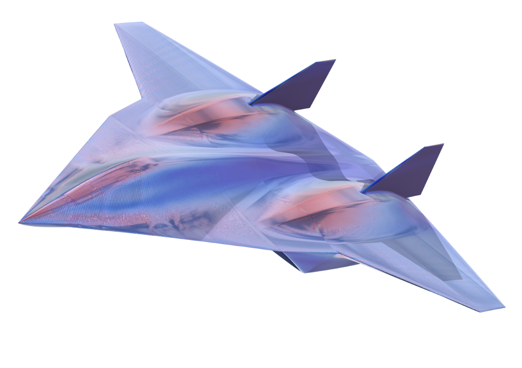
Figure 7. Surface currents on the Darkstar’s fuselage 1 GHz (left) and 3 GHz (right).
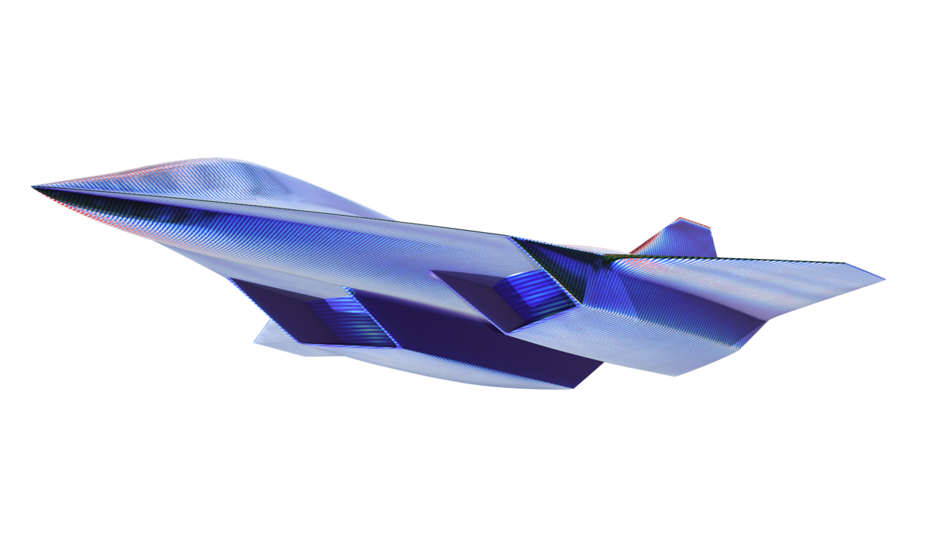
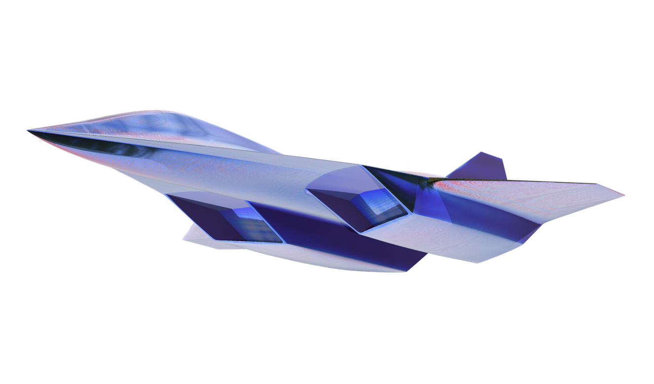
Figure 8. Surface currents on the Darkstar’s fuselage at 1 GHz (left) and 3 GHz (right), shown from an angle from below.
The mesh required to resolve the electromagnetic wave is rather dense. This is because we need at least five elements to resolve a wavelength, which means that an element cannot be longer than 2 cm for the case of 3 GHz.
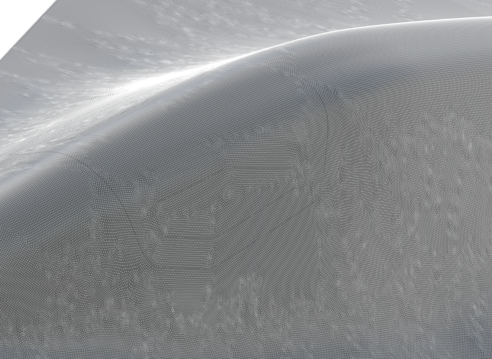
Figure 9. The mesh is so dense that it is difficult to see the elements without zooming in.
Figure 10 shows the radar cross section at 1 GHz and 3 GHz, computed as dB using 1 m2 as a reference. The backscattering half of the plot is what is reflected back to the enemy’s radar for detection of the approaching Darkstar. All of the values are well within the semicircle, which has a value of 0 dB and is equivalent to 1 m2. In fact, the highest values, displayed at 1 GHz, correspond to a value of -5 dB (0.3 m2). The values displayed at 3 GHz are below -10 dB (0.1 m2), which is of the order of magnitude of other stealth jets. The radar cross section is probably even smaller in the X-band, around 10 GHz, which would make the Darkstar even more difficult for the enemy’s missiles (it is probably flying too fast anyway).
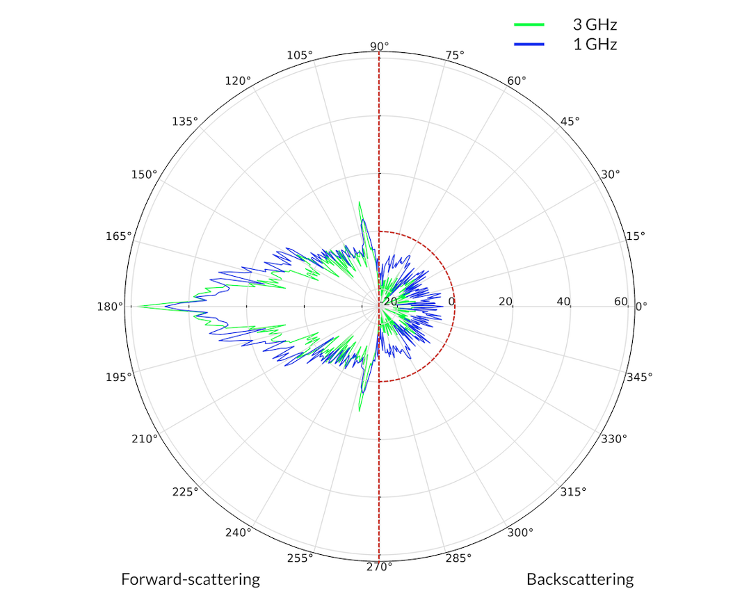
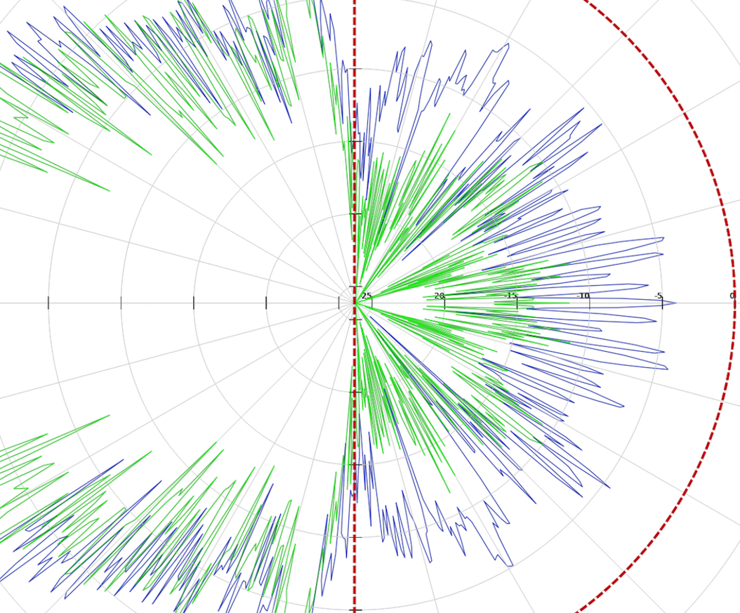
Figure 10. Radar cross section polar plot at 1 GHz and 3 GHz from a frontal aspect in a horizontal plane (left) and a close-up of the backscattering part of the plot (right).
It’s important to note that if we had a precise description of the geometry, the computed radar cross section would be more accurate. For example, details of sensors, a forward-facing radar, and the cockpit with its instrument panel would have an impact. On the other hand, the Darkstar would probably be covered with a radar-absorbent material, which would decrease its radar cross section. We actually applied such a paint to the engine air intakes in our simulations, but nowhere else. In addition, a plasma would likely form on the surface of the Darkstar due to it traveling at hypersonic speeds, which would also impact the radar cross section. What simplifies things somewhat is that the Darkstar would fly in scramjet mode during missions, closing the intake of the turbines. The turbines would otherwise reflect radar and would have to be included in the model.
In the above simulations, we used the boundary element method in COMSOL Multiphysics® and the RF Module. By using the Electromagnetic Waves, Boundary Elements interface we were able to account for edge scattering, creeping waves, and cavity return, which are not accounted for when using simpler physical optics methods.
Extending the Models and Watching the Movie
As mentioned, a general way of making the models discussed in this blog post more accurate would be to increase the level of details in their geometries. This would impact both the CFD and electromagnetic wave simulations. Improving the Darkstar’s geometry for accuracy would require adding sensors and incorporating small gaps and overlaps between the various metal plates forming the Darkstar’s fuselage, as well as including the necessary gaps and details for the cockpit entrance, windows, and landing gear doors. In addition, internal details of the airplane may also be important to include, such as the internal structure that is not shielded by metal, the nose cone radar, and the cockpit with the instrument panel. The extremely hot exhaust from the engines will probably also reflect the radar signal. Lastly, it’s important to note that the sweeping surfaces of the Darkstar’s fuselage, fins, and wings are complex, challenging to reproduce accurately, and crucial for both the CFD and electromagnetic wave simulation results.
Our analysis contains all of the components of a real modeling and simulation investigation. However, it was done for fun and to still our curiosity. A high-fidelity analysis would require many months of work by airplane designers, CAD, CFD, and radar specialists.
Now it’s time to return to the movie and get past its truly awesome start. I will try to avoid thinking about modeling and simulation this time…
More Blockbuster Content
Explore other modeling and simulation examples inspired by the media and entertainment industry on the COMSOL Blog:
- Defeating Giant Movie Monsters Using Mathematical Modeling
- What Is the Physics Behind a Counterweight Trebuchet?
The Darkstar and the scenarios discussed here are fictional elements from and/or inspired by the Top Gun movies.


Comments (2)
Jean-Marc Petit
April 9, 2024 COMSOL EmployeeGreat post ! I wonder about computational time for CFD ? and also thinking about heating at this speed since the airplane is in the air ?
Malgosia Zalewska
May 12, 2024How I can get a mph file for CFD model?