Pi on a String: An Interactive App to Estimate Pi

It’s easy to think of pi as a mathematical entity that lives only in circles and trigonometry, but this famous constant shows up in unexpected places. In this article, we simulate a seemingly modest device that can be used to estimate pi: a pendulum. Beneath the familiar oscillation lies a fascinating link between mathematics and physics. We bring this idea to life with a simple app that lets us easily experiment with different parameters and see the math in motion.

History of Estimating Pi

Historically, pi has been calculated through a variety of geometric methods by several ancient cultures. Later, during the 17^th and 18^th centuries, infinite series like the Gregory–Leibniz and Machin-like formulas advanced pi calculations, allowing mathematicians to compute up to hundreds of digits by hand.

Using modern technology, the calculation of pi has reached extraordinary precision using powerful computers and advanced algorithms. In a previous blog post, we discussed how the Monte Carlo method can also be used to estimate the value of pi. Today, state-of-the-art calculation methods involving rapidly converging infinite series, such as those derived from Srinivasa Ramanujan and the Chudnovsky brothers (Ref. 1), have allowed us to compute trillions of digits of pi.

The Simple Pendulum

In this blog post, however, we are moving away from sophisticated technology and will instead rely on an experiment you can easily replicate in real life. A simple pendulum consists of a mass (ideally point-like) called a bob, attached to one end of a string (ideally massless). The time period t of such a pendulum’s swing, which is the time it takes to complete one oscillation back and forth, can be formulated as

where L is the length of the pendulum and g is the acceleration due to gravity. If the time period of a pendulum’s swing is known, the value of pi can be estimated as

By measuring the time period of a pendulum’s oscillations, you can estimate the value of pi from direct observation. The equation assumes that the motion is simple harmonic — which is only true when the angle is small enough that sin⁡θ ≈ θ — so it works best for small release angles. You may notice that the time period is evidently independent of the mass of the bob. In realistic systems, however, the string will have a nonzero mass and the bob will have a nonzero radius. This means that the accuracy of the estimated value of pi improves when the pendulum mimics an ideal case, i.e., when the string is massless, when all of the mass is concentrated at a point-like bob, and when the initial angle is small (<15 degrees). 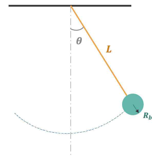A pendulum comprising a string of length L and a bob of radius R_b being released at an initial angle θ.

Building the Simulation App

A simulation app based on a COMSOL model can serve as a predictive tool, allowing you to explore how different design parameters, such as pendulum length or mass, affect the results before performing the actual experiment. To build a model of a simple pendulum, we’ll use the Multibody Dynamics interface, available in the Multibody Dynamics Module add-on product, as shown in this example model of a double pendulum. In the model the Events interface is used to track the number of oscillations in the simulation using a Discrete State variable called count. The process occurs in two stages, represented by two implicit events. When the bob’s velocity in the x direction becomes negative, count is incremented by a positive fractional value less than one. When the x-component of the velocity becomes positive again, count is rounded up to the next integer using the ceiling function. A stop condition is implemented as another implicit event that is triggered when count reaches the specified number of oscillations. Once the simulation terminates, the total simulation time (T_sim) and the number of oscillations (N) are used to calculate pi according to the equation

Now let’s use the Application Builder to create an app that estimates pi for different configurations of the simple pendulum. You can easily build custom simulation-based apps without needing extensive programming by using the drag-and-drop form design and the Method Editor for short code snippets. The app serves as an interactive tool to estimate pi for different pendulum parameters by computing the time period. This approach makes it especially useful in educational settings. For instance, a teacher could use the simulation to design a pendulum of appropriate size and timing for classroom demonstrations, helping students connect theoretical predictions with hands-on measurement. 

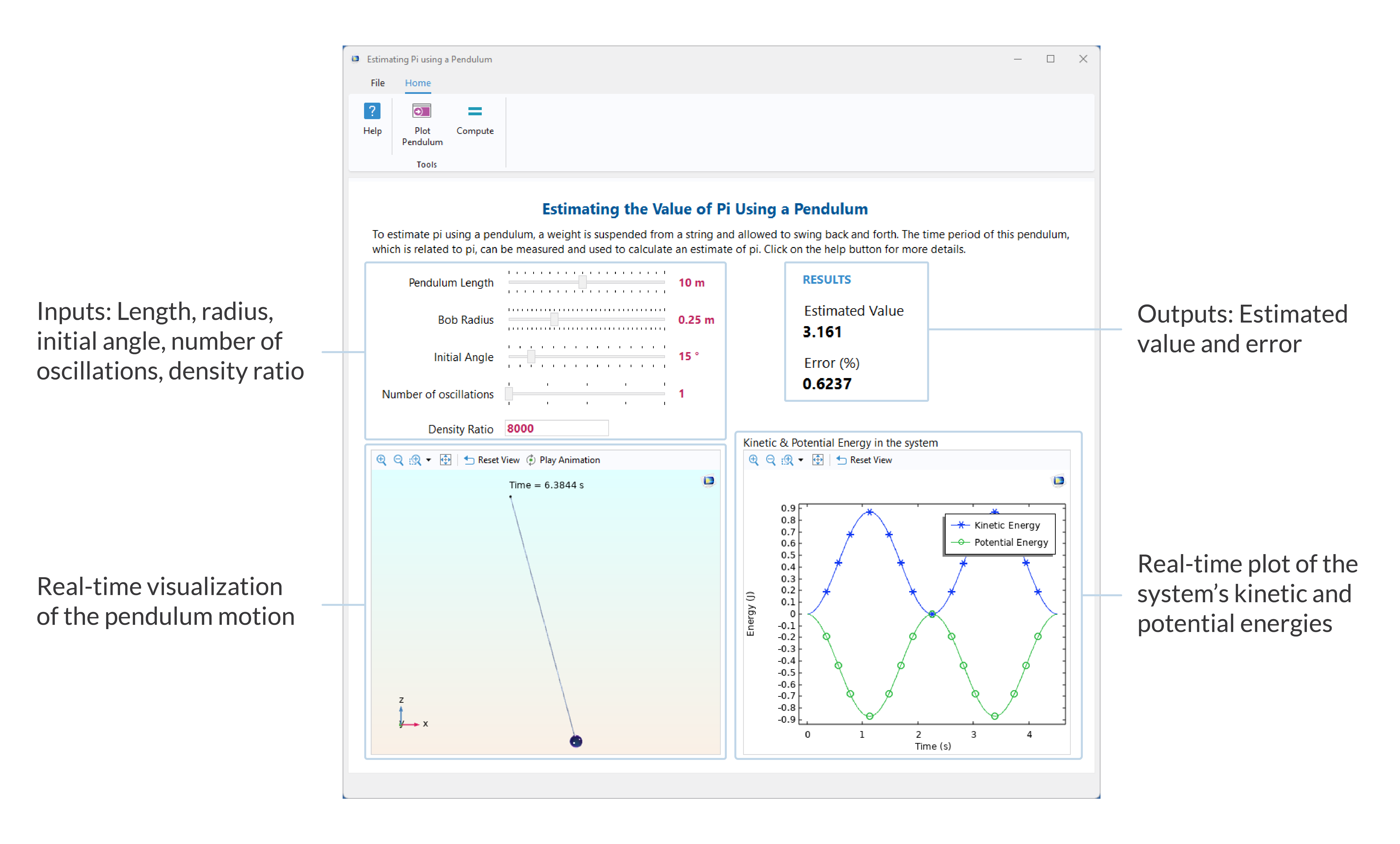The app’s UI.

The app contains sliders to control the length of the pendulum, the radius of the bob, the initial angle of release, and the number of oscillations to solve. It also contains a field where you can provide a numeric value of the ratio of the bob’s density to that of the string. 

Once you have chosen the desired parameters for your pendulum, clicking the Plot Pendulum button displays what your pendulum looks like based on the chosen values. The Compute button can then be used to simulate the pendulum, during which the Graphics window and the energy plot are updated in real time. After the solve, the estimated value of pi and the error from the true value are displayed to reflect the results obtained from the current solve. Feel free to share the set of input values that gave you the best estimate of pi in the comment section below!

A screen recording of the app in use.

Building an app like this in the COMSOL Multiphysics^® software using the Application Builder can be done by leveraging templates and without extensive programming experience. This way, engineers and scientists can link theory and simulation practically to make their models accessible to users who are not familiar with modeling.

Further Reading

Want to see how simulation apps are being used in the real world? Check out a few examples below:

• Read about a smartphone app powered by multiphysics simulation: Forecasting Fruit Freshness with Simulation Apps
• Take a look at how a university professor uses apps within the classroom: Bringing Lab Courses to Remote Learning Students with Simulation Applications

Reference

1. Borwein, J.M. and Borwein, P.B., 2004. Ramanujan and Pi. In Pi: A Source Book (pp. 588-595). New York, NY: Springer New York.