
In recent posts, we have covered a variety of plot types used for postprocessing simulation results in COMSOL Multiphysics and the ways that they can help you understand and share your results. Now let’s take a look at some tricks to simplify work in the graphics window.
Hidden Gems of the COMSOL Software Environment
Layering Plots
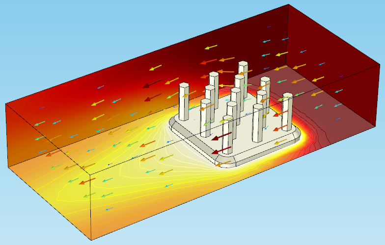
One helpful technique (which we’ve occasionally shown in other posts, but haven’t explicitly named) is to layer different surfaces together in a single plot group. This allows you to view several different results at once. For instance, you can combine plots that show the temperature and fluid flow for a CFD model, or show both the stress and deformation in a simulation of fluid-structure interaction. Let’s take the example of an aluminum heat sink, which was shown in this blog post on using surface, volume, and line plots. The plot below shows the temperature in the heat sink and the surrounding domain:
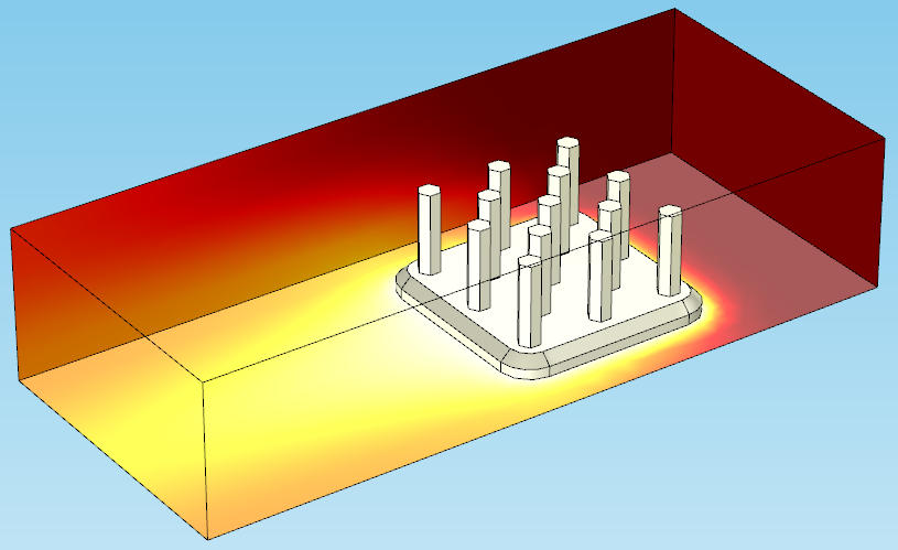
Adding a second plot simply requires right-clicking on the plot group node and choosing the next plot type you want. The new plot will be added on top of the first one and shown in the results tree. For this example, we can also add an arrow plot showing the fluid flow field past the heat sink:
![]()
After adding a second plot, the plot group node looks like this (and the arrow volume contains a color expression, not shown):
![]()
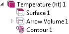
We can also add, for instance, a contour plot to see the temperature variation more clearly around the heat sink:

That addition makes the plot group tree look like this:
Note that there is no limit to the number of plots that can be added to a plot group, although it’s important to make sure that the plot doesn’t get too crowded. In certain cases, plots may interfere with each other — for example, it wouldn’t make sense to include a surface plot of the fluid flow velocity directly on top of the temperature plot, because it isn’t possible to see both at once. Even in this case, the contour and the arrow plots together make it look a little too busy.
Style Inheritance
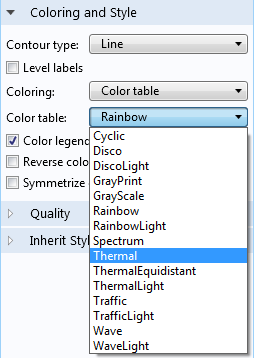
In the previous example, you might have noticed that the contour plot showing the temperature lines around the base of the heat sink has a different color scheme than the surface plot showing the temperature in the heat sink and surrounding domain. This could become confusing, especially since the rainbow color table is used in the arrow plot — which is showing fluid flow, not temperature. So as not to be misleading, we can change the two temperature plots to have the same color scheme (and make sure it’s different than the color scheme for plots showing other physics).
The obvious way to do this is simply to change the color table in the settings for each plot. In this case, we can change the contour plot to the thermal color table:
However, for a case where there are many subplots or there might be frequent changes made to style choices, it’s more beneficial to use the Inherit Style options. These enable you to inherit the style settings from a previous plot. We can set the contour plot to inherit its style from the temperature surface, locking the color settings in the contour plot unless we reset the inherit options:
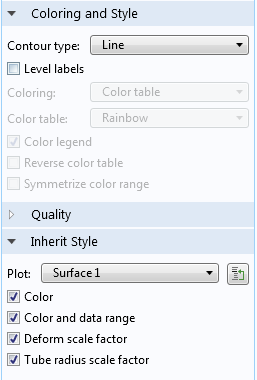
There are several checkboxes (shown above) that allow you to choose exactly which aspects of the plot’s style to keep. This is especially helpful for certain plot types where you have manually adjusted a setting — for instance, where a manual scale factor has been introduced and you want to make sure that all the successive plots maintain the scale.
Choosing to inherit the style from a previous plot also means that any changes made to the “parent” (the plot the settings are inherited from) will cause automatic changes in any plots relying on its style settings.
Enabling and Disabling Grid, Axes, and Legends
For COMSOL Multiphysics version 5.1, new buttons have been added to the graphics window toolbar that allow quick enabling and disabling of the grid, the coordinate axis symbol, and the color legends:
![]()
This means that it’s no longer necessary to go into the View node, and you can easily turn them off and on temporarily as needed.
Showing Mesh Plots
Another helpful tool (again shown in previous posts, but seldom discussed) is the Wireframe rendering option in the Coloring and Style tab. This checkbox allows you to display the mesh elements in a surface plot.
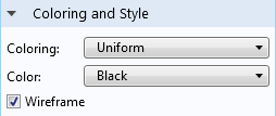
In many cases, it’s preferable to overlay two surface plots (as discussed earlier) so that there is a “background” for the mesh. For instance, in the heat sink, we might use a temperature surface on the heat sink, and then include a black mesh on top:
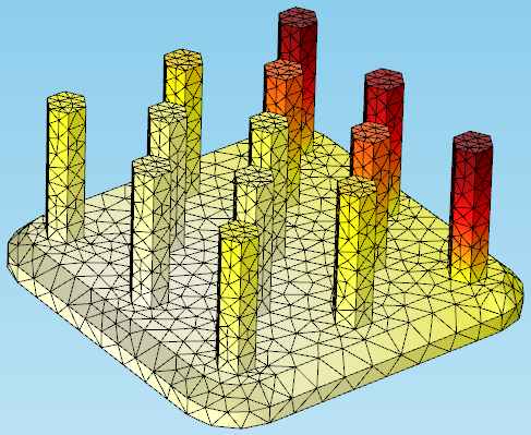
The mesh doesn’t have to be a uniform color (and will show an appropriate color gradient if a physics expression is used for the surface plot), but this feature is normally used with a gray or black mesh on top of a surface of a different color.
Exporting Results
COMSOL Multiphysics contains several options for exporting results such as images, animations, and reports. These are quite flexible and may be adapted to your specific needs.
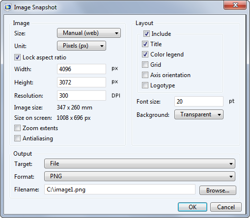
For exporting images from the graphics window, use the Image Snapshot button on the toolbar:
![]()
You can adjust the size and resolution, and control which aspects of the visible graphic are included in the image:
To create animations, right-click on the Export node and choose Animation. This will create a subnode where you can adjust the settings for a video to be exported to your chosen file type:
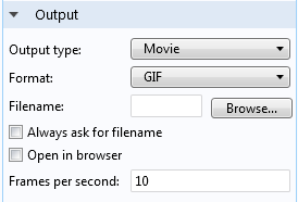
Among the settings are fields for controlling the number of frames, size, and speed of the video. Like the graphics export options, there are also choices for resolution and layout.
Note: The Player node is very similar to the Animation node (also accessible through the ribbon or by right-clicking on the Export node), except that it doesn’t save a file. Rather, this feature enables you to play and watch the animation directly in the graphics window.
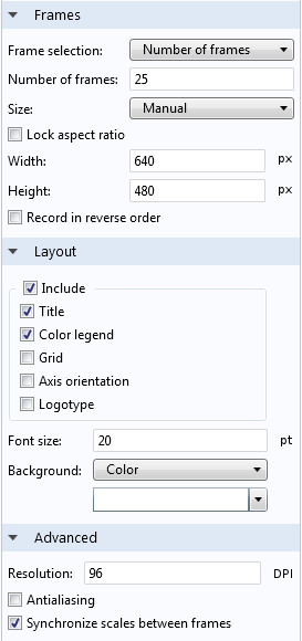
Finally, the Reports node allows you to generate a report of your results as an HTML or Microsoft® Word file. Several options are available for different amounts of detail, as well as a Custom Report option that lets you choose exactly which aspects of the simulation you’d like to include.
A complete report will include everything in the Model Builder, from the parameters table to the final results plots.
Rearranging the COMSOL Desktop
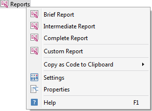
Lastly, a little-known fact about the COMSOL Desktop is that you can rearrange the windows using the drag-and-drop method. All of the windows below the ribbon can be moved and dropped into different sections. Release the mouse over one of the blue boxes to set it in the corresponding position (shown below):
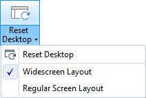
If you ever want to reset the Desktop layout, the Reset Desktop button on the ribbon will revert the windows to the default arrangement. This feature also allows you to choose between two different layouts, depending on the size of your window and monitor:
This completes our overview of using additional tricks and tools for postprocessing in COMSOL Multiphysics. We hope that you’ll find these techniques useful in your own work for visualizing, understanding, and sharing your simulation results. Thanks for reading!


Comments (0)