
The Doppler effect, or Doppler shift, occurs when the movement of an observer relative to a source (or vice versa) causes a change in wavelength or frequency. Discovered by Austrian physicist Christian Doppler in 1842, this phenomenon is experienced in many different ways, such as when an ambulance passes you by and you hear an audible change in pitch. Using the COMSOL Multiphysics® software, you can model the Doppler effect for acoustics applications.
The original version of this post was written by Alexandra Foley and published on July 15, 2013. It has since been revised with additional details, animations, and an updated version of the featured model.
The Doppler Effect, Explained
One of the most common ways we experience the Doppler effect in action is the change in pitch caused by either a moving sound source around a stationary observer or a moving observer around a stationary sound source. When the sound source is stationary, the sound that we hear is at the same pitch as the sound emitted from the sound source.
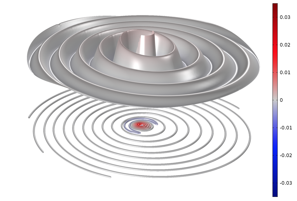
Sound waves propagating from a stationary sound source in a uniform flow (this corresponds to the source moving at constant speed).
When the sound source moves, the sound we perceive changes. Going back to the ambulance example, when an ambulance drives past us, the siren sounds different than it would if we were standing right next to it. The moving ambulance has a different pitch as it approaches, when it is closest to us, and as it passes us and drives away.
As the ambulance moves toward us, each successive sound wave is emitted from a closer position than that of the previous wave. Because of this change in position, each sound wave takes less time to reach us than the one before. The distance between wave crests (the wavelength) is thereby reduced, meaning that the perceived frequency of the wave increases and the sound is perceived to be of a higher pitch. Conversely, as a sound source moves away, waves are emitted from a source that is farther and farther away. This creates an increased wavelength, a decreased perceived frequency, and a lower pitch.
The situation is mirrored when we drive by the siren of an ambulance that is parked. In this instance, the observers (us) move toward the source (the siren) and the sound waves reach us from closer and closer positions as we move.
Visualizing Another Example of the Doppler Effect
Another example of the Doppler effect that is easy to visualize involves waves on a water surface. For instance, a bug rests on the surface of a puddle. When the bug is stationary, it moves its legs to stay afloat. These disturbances propagate outward from the bug in spherical waves.
When the bug starts moving across the water, the water flow around the bug changes. The waves appear closer together when we look at the bug swimming toward us (eek!) and farther apart as it swims away (phew!) The animation above shows the principle for waves (ripples) on water, which move much slower than the speed of sound. The slower speed is why, in this instance, the Doppler effect can be seen with the naked eye.
Simulating the Doppler Effect
By using the COMSOL Multiphysics® software and the add-on Acoustics Module, you can simulate the Doppler effect and measure the change in frequency for a source moving at a certain velocity. Let’s assume that the air surrounding the sound source (the ambulance, in this case) is moving with a velocity of V = 50 m/s in the negative z direction. We also assume that the observer of the sound is standing 1 m from the ambulance as it passes by. In the figure below, we can see the change in the pressure as the ambulance approaches and passes an observer.

In this plot, the distance of the ambulance from the observer is represented on the x-axis. The solid line represents the pressure perceived by the observer of an approaching ambulance and the dashed line shows the pressure as the ambulance gets farther away.
From this plot, we can see how the amplitude of the wave (or pressure) drops off at a faster rate when the ambulance is moving away from an observer compared to when it approaches. The change in the amplitude of the wave depicts how the siren becomes quieter as the ambulance moves away. The rate at which the sound level decreases as the ambulance recedes is much faster than the rate at which the sound becomes louder as the ambulance approaches (as shown in the graph above).
To look at this effect in a different way, we can visualize the sound pressure level around the sound source (remember, the source is effectively moving in the positive z direction).
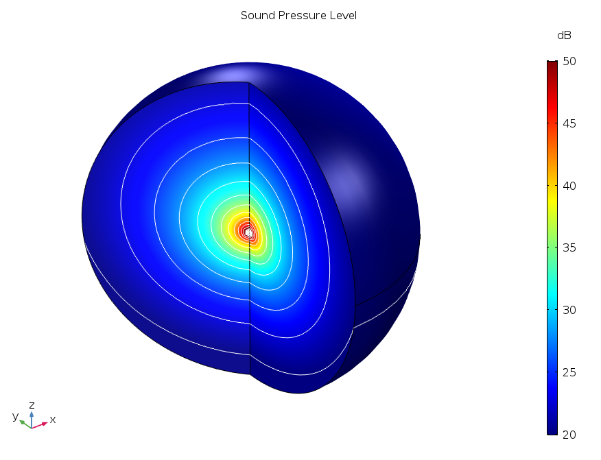
The sound pressure level around the sound source is represented by colors and contour lines. You can see how the outermost contour runs from well inside the physical domain to the perfectly matched layer, showing that the sound is greater below the source than above it.
Other Examples of the Doppler Effect
The Doppler effect is apparent in many other phenomena. One common example is Doppler radar, in which a radar beam is fired at a moving target. The time it takes for the beam to bounce off the target and return to the transmitter can provide information about a target’s velocity. Doppler radar is used by police to identify people driving faster than the speed limit.
The Doppler effect is also used in the field of astronomy to determine the direction and rate at which a star, planet, or galaxy moves compared to Earth. By measuring the change in the color of electromagnetic waves — called redshift or blueshift — an astronomer can determine a celestial body’s radial velocity. If you notice a star that appears red, it is quite far from Earth — and a visible sign that the universe is expanding!
Other applications that take advantage of the Doppler effect include meteorological forecasts, sonar, medical imaging, blood flow measurement, and satellite communication.
Next Steps
Click the button below to try simulating the Doppler effect. You will be able to download the MPH file for the example featured in this blog post.
Additional Resources
- Learn about the man who discovered the Doppler effect in this blog post on Christian Doppler
- Explore the Acoustics Module


Comments (0)