Fluid Flow: Conservation of Momentum, Mass, and Energy
Describing Fluid Flow
There are various mathematical models that describe the movement of fluids and various engineering correlations that can be used for special cases. However, the most complete and accurate description comes from partial differential equations (PDEs). For instance, a flow field is characterized by balance in mass, momentum, and total energy described by the continuity equation, the Navier-Stokes equations, and the total energy equation:
(1)

The solution to the mathematical model equations gives the velocity field,  ; pressure, p; and temperature, T; of the fluid in the modeled domain.
In principle, this set of equations is able to describe flows from the creeping flow in a microfluidic device to the turbulent flow in a heat exchanger and even the supersonic flow around a jet fighter. However, solving Equation (1) for a case such as the jet plane shown below is not feasible and while it is possible to solve the whole of Equation (1) for a microfluidic device, it is a lot of work down the drain. Much of computational fluid dynamics (CFD) is therefore devoted to selecting suitable approximations to Equation (1) so that accurate results are obtained with a reasonable computational cost.
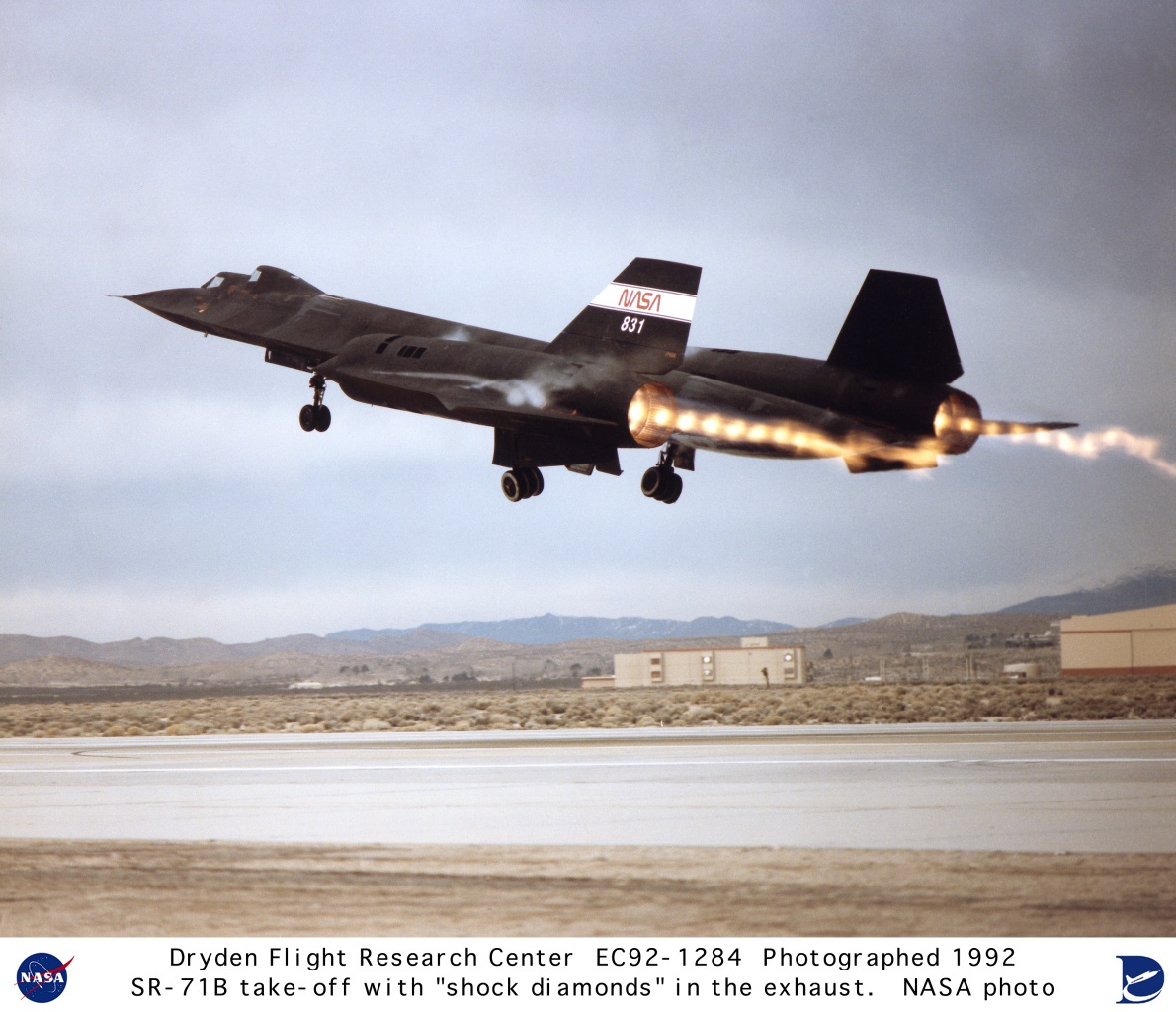
SR71 supersonic jet. The exhaust forms shock diamonds typical for supersonic flows. Image in the public domain via the Dryden Flight Research Center, NASA.
SR71 supersonic jet. The exhaust forms shock diamonds typical for supersonic flows. Image in the public domain via the Dryden Flight Research Center, NASA.
The Continuum Hypothesis and Rarefied Flows
The flow equations (Equation (1)) rely on the continuum hypothesis, that is, a fluid can be regarded as a continuum rather than a collection of individual molecules. Flows where molecular effects are of significance are known as rarefied flows. The degree of rarefaction is measured by the Knudsen number:

where  is the molecular mean free path and L is a representative length scale for the flow geometry; for example, a channel width.
A flow can be regarded as a continuum flow as long as the Knudsen number is smaller than 10-3. Liquids can almost always be regarded as continua, as can gases under ordinary circumstances. For gases at very low pressures, or gas flows confined in very small domains, the interaction of the molecules in the fluid may take place with the same frequency as the interaction with the walls that confine the flow. For such systems, the fluid flow has to be described with the rarefied flow equations or at least with Knudsen boundary conditions.
Newtonian and Non-Newtonian Fluids
A fluid is characterized by, among other things, its viscosity. The viscous effects are contained in the viscous stress tensor,  . Most commonly encountered fluids, such as water, gases, and ethanol, are Newtonian. For Newtonian fluids, the viscous stress is proportional to the deviatoric stress tensor:

There are, however, a number of fluids that do not obey the simple relation in Equation (3). Such fluids are known as non-Newtonian and can display a wide range of behaviors. Examples of non-Newtonian fluids include blood; paint; some lubricants; cosmetic products; food products such as honey, ketchup, juice, and yogurt; and many suspensions, for example sand in water or starch suspended in water.
Honey is an example of a non-Newtonian fluid.
Incompressible Fluid Flow
A fluid can be regarded as incompressible if the density variations are very small; that is, if  . This is true for liquids (unless there are significant temperature variations) and gases under moderate pressure and temperature variations. If we can neglect the heating due to viscous dissipation (so-called viscous heating) and assume that the fluid is Newtonian, Equation (1) can be simplified to:

The middle equation in Equation (4) is the famous Navier-Stokes equation, named after the French physicist Navier and the Irish physicist Stokes. Navier was first to derive the equations, but the understanding of the physical mechanism behind the viscous term was first explained by Stokes, hence the name of the equations.
In some cases, the first equation, the continuity equation, is also included in the Navier-Stokes equations. As can be seen, the energy equation has been rewritten as a temperature equation, which is much more convenient to work with. The temperature equation is for incompressible flows completely decoupled from the Navier-Stokes equations, unless the viscosity depends on the temperature.
The solution to the Navier-Stokes equations gives the velocity and pressure field for flows of fluids with constant viscosity and density. The temperature can be solved for separately if information about the temperature field is desirable.
Buoyancy is an important physical phenomenon that formally comes from variations in density. Equation (4) can, however, still be used to model the effect of buoyancy by introducing buoyancy as a momentum source/sink in the momentum equations.
Even in cases where there is nonconstant density, the Navier-Stokes equations may be used and the effect of buoyancy may be introduced as a momentum source/sink in the momentum equations. For example, buoyancy makes the smoke from a cigar flow upward.
The Reynolds Number
A central concept in fluid flow is the Reynolds number. It is defined as:

where U is a representative velocity scale and L is a representative length scale.
In absence of body forces, and if the density and the viscosity are constant, the Navier-Stokes equation (middle expression in Equation (4)) can be nondimensionalized to read:

where  , with
  being a representative pressure level.
As can be seen from Equation (6), the Reynolds number measures the relative importance of the viscous stresses. A low Reynolds number means that the flow is completely governed by viscous effects, while the flow is effectively inviscid at very high Reynolds numbers.
Observe that there can be several Reynolds numbers associated with a particular flow configuration. A channel flow, for example, can be based on the channel half width or the whole channel width. The velocity can either be the average velocity or the maximum velocity. Therefore, it is important to know which length scale and velocity scale are associated with a particular Reynolds number, especially when comparing Reynolds numbers between similar flow configurations.
Stokes Flow
Flows at very low Reynolds numbers are known as creeping flows. They can be encountered in, for example, microfluidic systems (such as the micromixer shown below) or lubrication systems.
 The Stokes equations are often used to model flow in microfludics, such as the flow in this micromixer.
The Stokes equations are often used to model flow in microfludics, such as the flow in this micromixer.
The Stokes equations are often used to model flow in microfludics, such as the flow in this micromixer.
The limit when  is known as Stokes flow. Stokes flow can formally support both time dependency and varying material properties, but classical Stokes flow is written for incompressible quasistatic conditions:

The equations are named after the Irish physicist George Gabriel Stokes, who first described viscous momentum transfer through these equations. Which terms to retain from the energy equation depends on the fluid. The convective term can often be neglected, as can pressure-work effects. Viscous heating can also be of interest for Stokes flows in bearings and other lubrication applications, for example.
Turbulent Flow
The Reynolds number measures the importance of the inertial effects compared to the viscous effects. As long as the Reynolds number is not too large, the viscous effects will damp out perturbations in the flow field. Such flows are known as laminar flows. It is often feasible to solve, for example, Equation (4) for laminar flows, since the viscosity dissipates any flow structures that are small enough.
The higher the Reynolds number, the more inertial effects dominate over viscous effects. When the Reynolds number is high enough, any small perturbation will feed on the mean flow momentum and grow and trigger new flow structures. This phenomenon is called transition.
A flow that has undergone transition is denoted turbulent flow. Turbulent flows are characterized by the seemingly chaotic eddies that have a huge span of length scales, from the large vortices that can be almost as large as the computational domain down to the small dissipative eddies that can be as small as micrometers. This wide span of scales means that not many turbulent flows can be simulated at a reasonable computational cost using the pure Navier-Stokes equations. It is possible to perform so-called direct numerical simulation (DNS) for some very simple flow cases, but it requires vast computational resources.
In order to make it possible to estimate the flow and pressure fields without having access to a supercomputer, we usually introduce approximate turbulence models. The turbulence models formulate different types of conservation expressions for turbulence in an averaged sense; for example, by looking at the conservation of the kinetic energy that these small eddies may have (called turbulent kinetic energy). The conserved properties, such as the turbulent kinetic energy, are used to generate an additional contribution to the viscosity, called eddy viscosity. The eddy viscosity enlarges the viscous transfer of momentum in order to mimic the momentum that would be transferred by the small-scale eddies that we cannot afford to resolve.
The most common turbulence models used in engineering are the Reynolds-averaged Navier-Stokes models (RANS models), in which the modeled quantities are time-averaged and the fluctuations are treated in an introduced quantity referred to as the Reynold stresses. The RANS equations for incompressible flows read:

where bar denotes an averaged quantity and prime is the deviation from average.
The unfiltered velocity, for example, can be written  . Comparing Equation (8) to the continuity and momentum equations in Equation (4), it can be seen that the equations are identical except that unfiltered quantities have been replaced by filtered quantities, there is no time derivative (since we averaged over time), and there is an extra term
  in Equation (8). This term is the Reynolds stress tensor and represents the effect of the turbulent fluctuations on the filtered velocity and pressure fields.
It is possible to formulate transport equations for the entries in the Reynolds-stress tensor. With appropriate simplifications and assumptions, these equations can result in so-called Reynolds-stress models. While powerful, these models are often difficult to work with and even if they are computationally much less expensive than DNS, they are still too expensive for most industrial applications.
The most common approach is instead to assume that the turbulence acts as an additional viscous effect and write  , where
  is the turbulence viscosity, also known as the eddy viscosity. Models for the eddy viscosity include the most widely used models for industrial applications such as k-ε, k-ω, shear stress transport (SST), and the Spalart-Allmaras turbulence models.
There is another class of turbulence models that averages turbulence over a small spatial region instead of over time. This forms a sort of low-pass filter for eddies below a certain length scale. In this way, large turbulent eddies are resolved while the effect of small eddies have to be modeled, hence the name large eddy simulation (LES). The continuity and momentum equations for incompressible LES take the same form:

Equation (9) is identical to Equation (8), but with a time derivative. Also, the term is the subgrid stress (SGS) tensor and it represents the effect of the subgrid scales on the resolved scales. A commonly used model for the SGS tensor is the Smagorinsky-Lilly model.
LES is often more accurate than RANS, but the simulations must always be 3D, even if the flow is essentially 2D and the simulations are always time dependent. In addition, the required resolution for the SGS models to be valid is often quite high, which means that LES is only used when even the most advanced RANS models fail to capture the essential features of the flow.
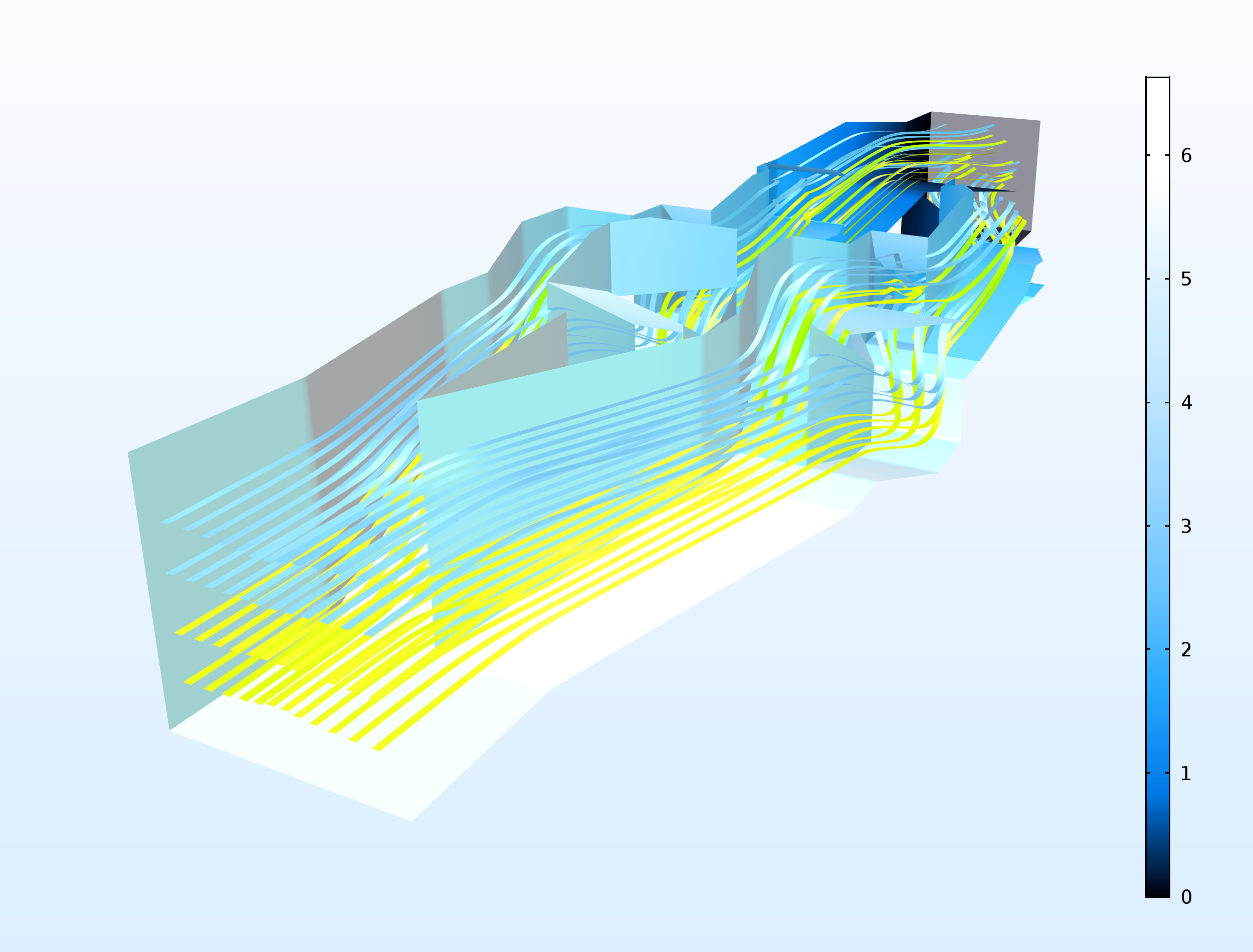
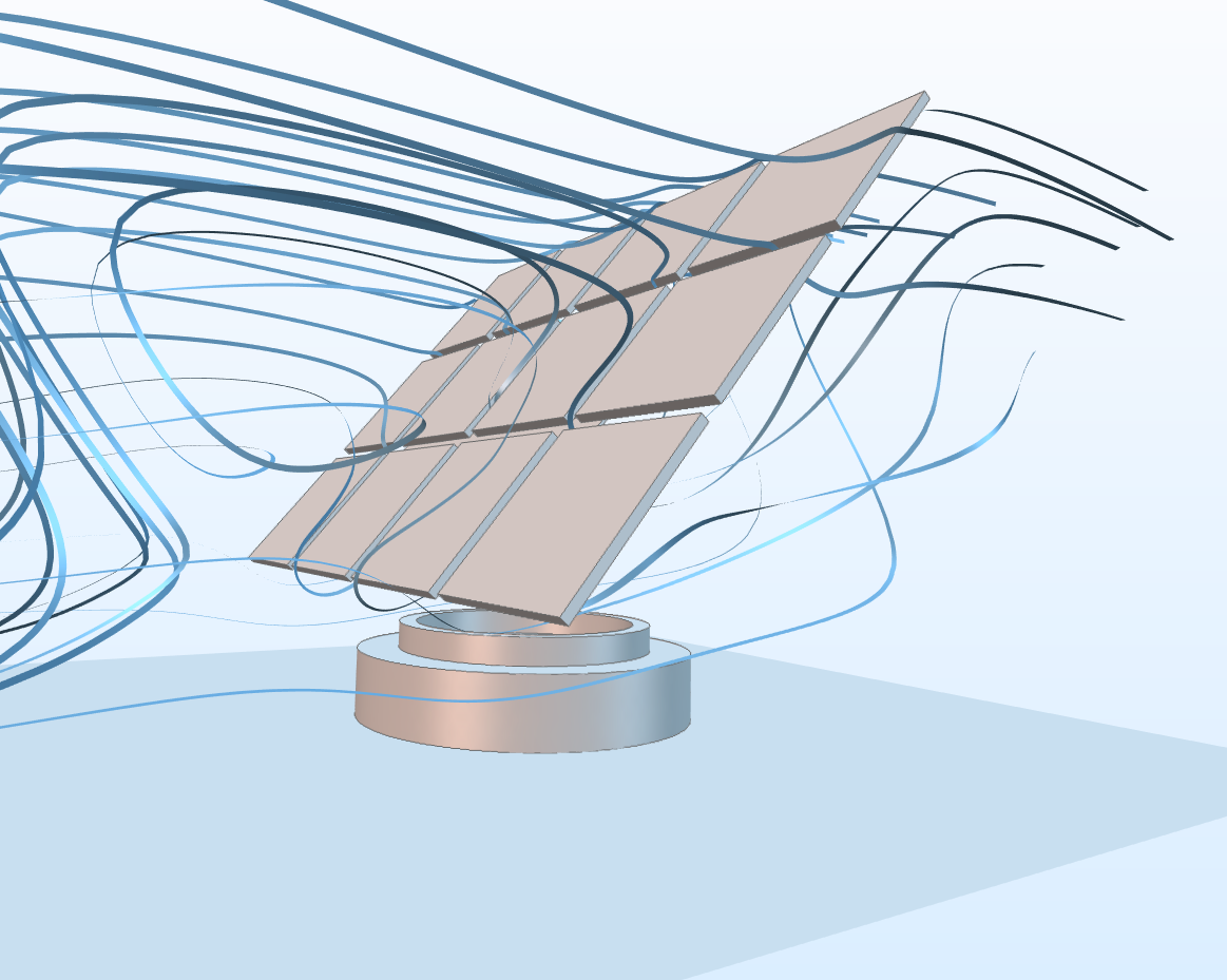 Turbulent wind flow around a solar panel. The low-Reynolds RANS turbulence models can be used to estimate the force that the panels are subjected to by the wind.
Turbulent wind flow around a solar panel. The low-Reynolds RANS turbulence models can be used to estimate the force that the panels are subjected to by the wind.
Turbulent wind flow around a solar panel. The low-Reynolds RANS turbulence models can be used to estimate the force that the panels are subjected to by the wind.
The Mach Number
The Mach number is defined as:

where c is the speed of sound.
The Mach number measures how fast a fluid moves compared to the speed of the pressure waves. When the Mach number is small, that is, when  , the pressure waves are so fast that they effectively reduce to a mass conservation constraint. The incompressible flow formulation in Equation (4) can formally be reached by letting
  . As the Mach number approaches 1 — that is, when the velocity approaches the speed of sound — the effects of the pressure waves must also be included. Viscous heating is also often important in these cases and the result is that we must solve the complete set of continuity, momentum, and energy equations given by Equation (1). Flow where all terms in Equation (1) are important is sometimes referred to as compressible viscous flow.
If the Mach number is high, then oftentimes, so too is the Reynolds number, as both are proportional to the velocity. So, Equation (1) is often complemented with a turbulence model to account for the eddy diffusivity for momentum eddy diffusivity for heat transfer. The coupling between Equation (1) and its turbulence model is often very strong.

Fully compressible turbulent flow modeled with the k-ε turbulence model. We can see the diamond-shaped pattern of the velocity field caused by the pressure shocks (shock diamonds).
Fully compressible turbulent flow modeled with the k-ε turbulence model. We can see the diamond-shaped pattern of the velocity field caused by the pressure shocks (shock diamonds).
Inviscid Flow and the Euler Equations
For flow of gases at moderate pressures close to and above the speed of sound, the contribution of molecular viscosity and eddy viscosity to the transfer of momentum can often be neglected. In such cases, the model equations describe the conservation of momentum (without a viscous term), the conservation of mass, and the conservation of energy. There is no need for a turbulence model, since the eddy viscosity is not accounted for.
In the energy equations, the analogy to viscous momentum transfer is heat transfer through conduction. In fact, in gases, the same mechanism that is responsible for viscosity is also responsible for thermal conductivity and the eddy diffusivity for momentum transfer is also used to compute the eddy diffusivity for heat transfer. Consequently, in cases where we can neglect viscous momentum transfer, we can usually neglect heat transfer through conduction in the energy equations.
The conservation equations for inviscid flow and negligible thermal conductivity are usually referred to as the Euler equations after the famous Swiss mathematician who first formulated them. The Euler equations read:

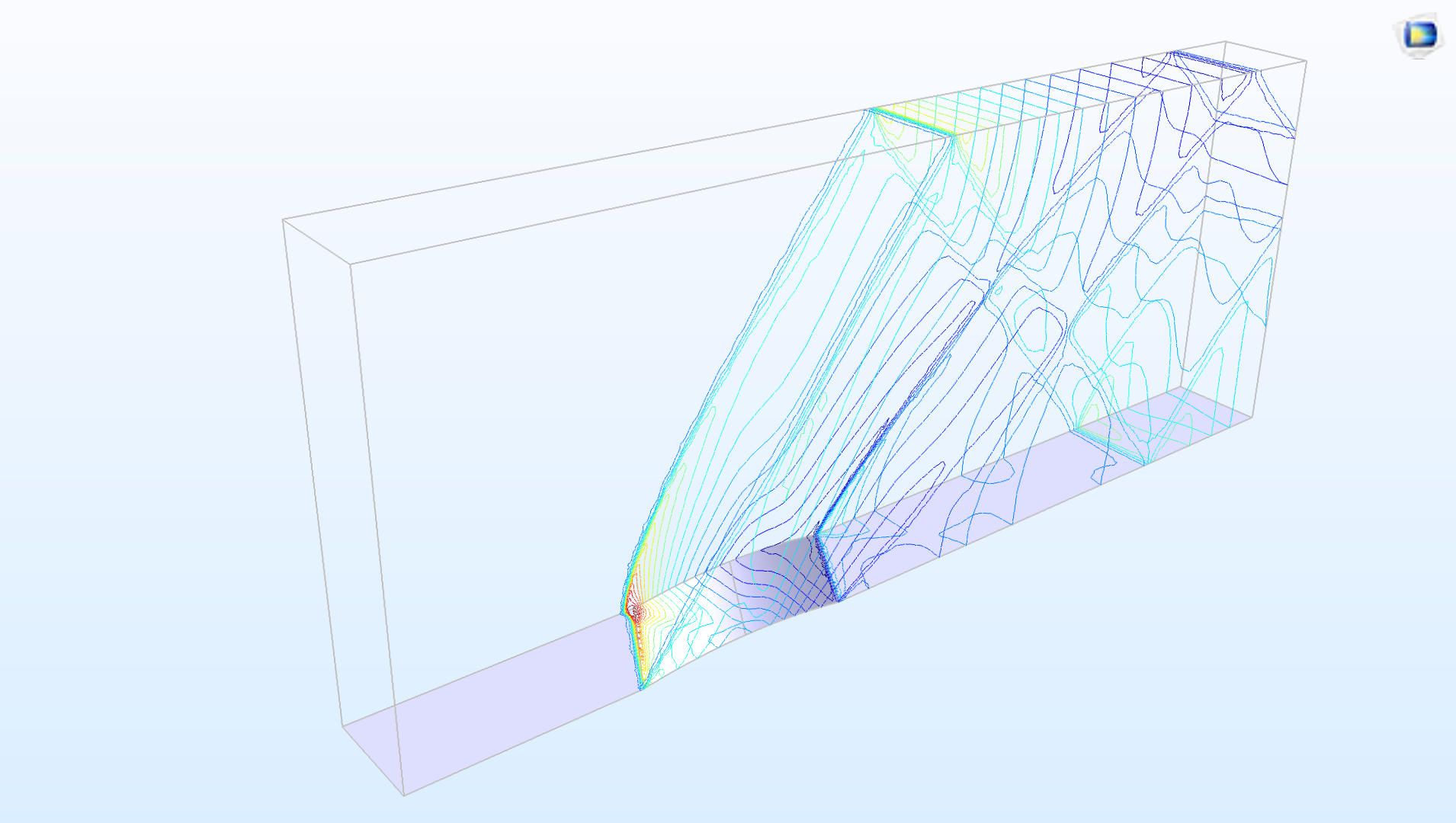 Supersonic flow over a wing-shaped obstacle that causes pressure shocks, which reflect on the walls of this benchmark problem for the solution of the Euler equations for high Mach number flow.
Supersonic flow over a wing-shaped obstacle that causes pressure shocks, which reflect on the walls of this benchmark problem for the solution of the Euler equations for high Mach number flow.
Supersonic flow over a wing-shaped obstacle that causes pressure shocks, which reflect on the walls of this benchmark problem for the solution of the Euler equations for high Mach number flow.
Multiphase Flow
The equations for the conservation of momentum, mass, and energy can also be used for fluid flow that involves multiple phases; for example, a gas and a liquid phase or two different liquid phases, such as oil and water.
The most detailed way of modeling multiphase flow is with surface tracking methods, such as the level set or phase field methods. In these models, the interactions between phases — for example, surface tension — are introduced as sources or sinks in the momentum equations at a thin layer with a very small thickness that follows the boundary between the phases. The shape and position of the phase boundary is computed in detail. This means that the momentum and mass conservation equations are combined with a set of transport equations for a level set or phase field function that, at a given value (isosurface), describe the position of the phase boundary.
Classical benchmark model for surface tracking two-phase flow models. Note how for a very short moment, the heavier fluid gets attached to the top wall during sloshing. This attachment is due to surface tension.
When the phase boundary consists of millions of droplets or bubbles, or when the shape of the phase boundary is very complex in its details, we cannot computationally afford to track its shape. Instead, we have to make some kind of homogenization and treat the presence of the different phases as fields of averaged mass or volume fractions. We no longer track the shape of the phase boundary in detail. Instead, we introduce the possible interactions between the phases as momentum sources and sinks defined everywhere in the fluid mixture. In addition, the conservation equations for momentum and mass are combined with a transport equation for the volume fraction for one of the phases in the case of two-phase flow and two transport equations for three-phase flow. When there is a large difference in density between two phases, we may even have to formulate separate momentum equations for each phase defined everywhere in the fluid domain.
For bubbles in liquids, a dispersed flow model such as the bubbly flow model may give a good representation of the homogenized two-phase flow. For liquid-liquid solutions, such as oil and water, we may use a slightly more complex model, such as the mixture model for multiphase flow.
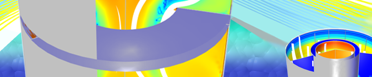
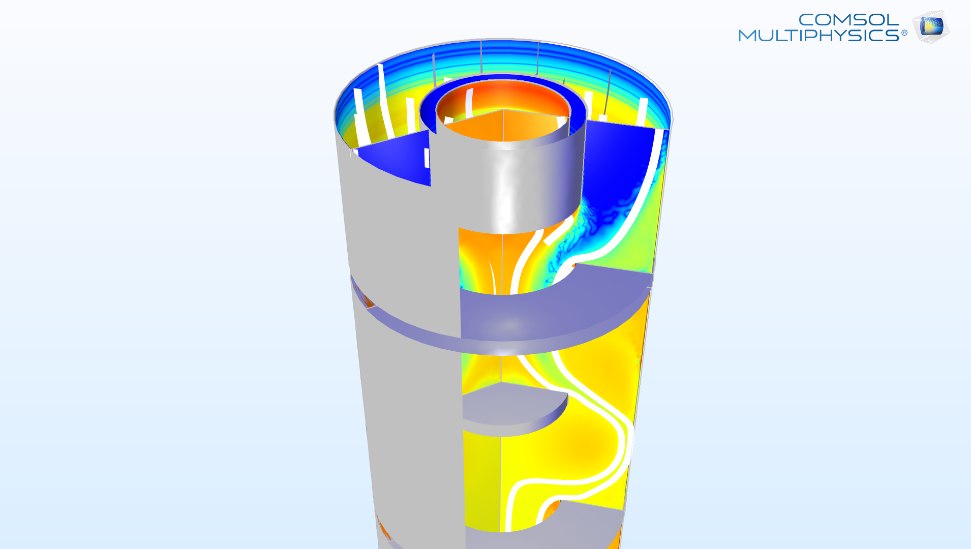 Model of a liquid-liquid extraction column. The plot shows the volume fraction of oil. The heavier water solution enters at the top annular inlet, while the oil phase exits at the top circular outlet.
Model of a liquid-liquid extraction column. The plot shows the volume fraction of oil. The heavier water solution enters at the top annular inlet, while the oil phase exits at the top circular outlet.
Model of a liquid-liquid extraction column. The plot shows the volume fraction of oil. The heavier water solution enters at the top annular inlet, while the oil phase exits at the top circular outlet.
For a large number of solid particles in a gas, where the difference in density is very large, we often need to formulate the momentum equations for both the dispersed solid particles and the gas phase. Models that define the momentum equations for each phase are usually referred to as Euler-Euler multiphase flow models. The name comes from the fact that both phases are described as continua, that is, by an Eulerian approach.
When the particles are few enough, an alternative option is to use a particle tracking method to describe the dispersed phase. This is known as the Euler-Lagrange method, since the continuum (for example, the fluid) is described by an Eulerian approach, while the particles are described by a Lagrangian approach. The advantage of the Euler-Lagrange method is that properties can then be associated with each individual particle, but the method becomes very expensive as the number of particles increases.
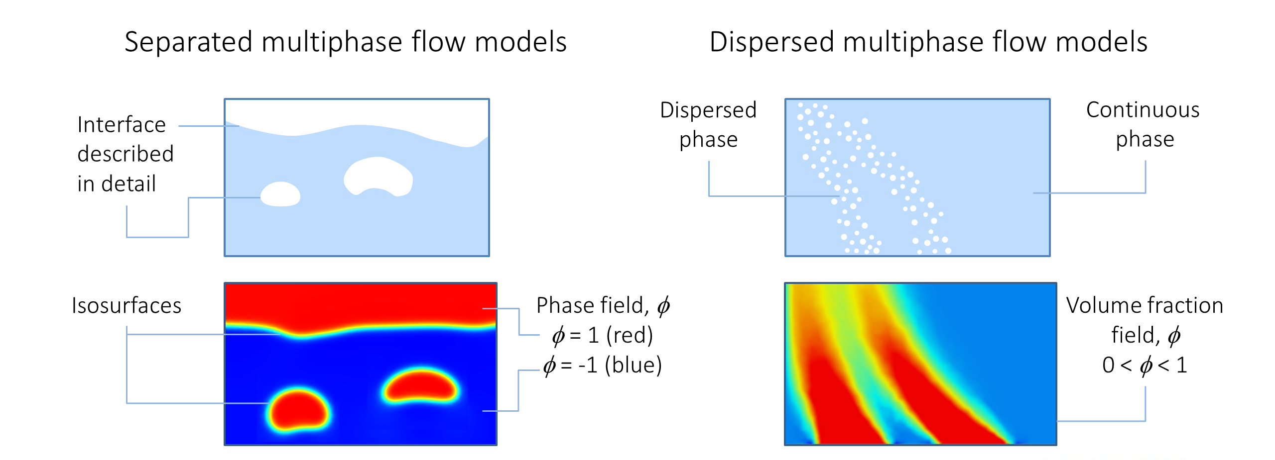 The difference between separated multiphase flow models that use surface tracking methods (left) and dispersed multiphase flow models (right). In the surface tracking method, the isosurface of the field φ at φ = 0 represents the phase boundary. In the dispersed multiphase flow model, only the volume fraction of bubbles or droplets is obtained, while the details of the phase boundary are treated as averaged volume forces.
The difference between separated multiphase flow models that use surface tracking methods (left) and dispersed multiphase flow models (right). In the surface tracking method, the isosurface of the field φ at φ = 0 represents the phase boundary. In the dispersed multiphase flow model, only the volume fraction of bubbles or droplets is obtained, while the details of the phase boundary are treated as averaged volume forces.
The difference between separated multiphase flow models that use surface tracking methods (left) and dispersed multiphase flow models (right). In the surface tracking method, the isosurface of the field φ at φ = 0 represents the phase boundary. In the dispersed multiphase flow model, only the volume fraction of bubbles or droplets is obtained, while the details of the phase boundary are treated as averaged volume forces.
Porous Media Flow
If we can afford to describe a porous structure in detail, with all of its surface structures and surface properties, we can use the equations for the conservation of momentum and mass as usual, defining no-slip conditions on the pore walls or the Knudsen condition if the mean width of the pores is of the same order of magnitude as the scale of molecule interactions.
However, in most cases, we cannot afford to describe the millions of pore bends and structures in a macroscopic model of a porous structure. Therefore, models for porous media flow usually use homogenization in order to define the fluid and the porous matrix domains in the porous structure as a slab with averaged properties, such as averaged porosity, tortuosity, and permeability. The momentum equations then become Darcy’s law, named after the French engineer who first formulated this law. Darcy’s law may be extended with a shear term to form the Brinkman equations, named after the Dutch physicist H.C. Brinkman.
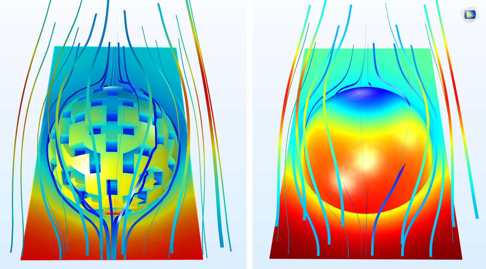 Flow over and through a porous particle, where the structure is described in detail (left) and the homogenized corresponding model (right).
Flow over and through a porous particle, where the structure is described in detail (left) and the homogenized corresponding model (right).
Flow over and through a porous particle, where the structure is described in detail (left) and the homogenized corresponding model (right).
Last modified: June 29, 2018