
Version 6.0 of the COMSOL Multiphysics® software extends the functionality of the Magnetic Fields, Currents Only interface within the AC/DC Module to compute stationary and frequency-dependent inductance matrices and AC resistances for electrical systems that are composed of nonmagnetic materials. This is useful for analyses of printed circuit boards and power bus systems. It is possible to compute total inductance as well as partial inductances. The partial inductance, however, requires a bit of understanding to interpret and use appropriately. Let’s learn more!
Defining and Computing Total and Partial Inductance
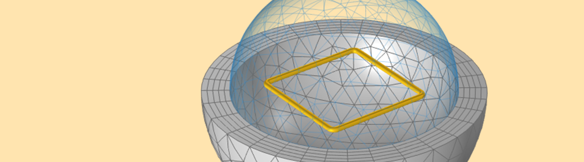
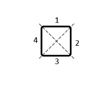
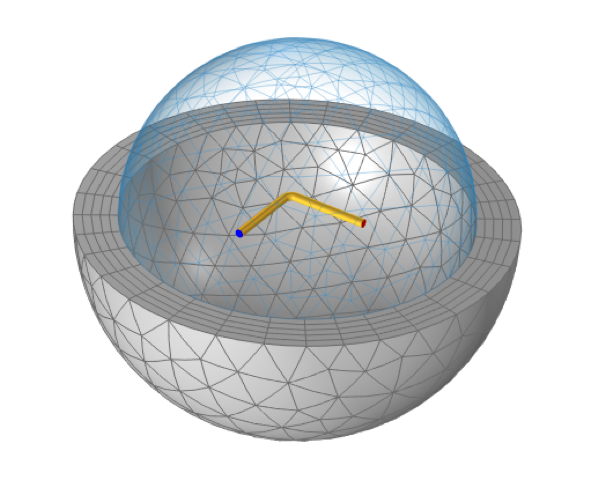
For the purpose of understanding total and partial inductances, let’s start by considering a model of a square loop of wire, as shown in the figure below. When current flows along this closed loop there will be a magnetic field in the surrounding space. We can define and compute the total inductance, L^{tot} (often referred to as simply “the inductance”), from the total stored magnetic energy in the modeling space, W_{m}^{tot}, and the current flowing through the coil, I, via: L^{tot} = 2 W_m^{tot}/I^2. This square loop, with a wire diameter of 1 mm and a side length of 2 cm, has a total inductance of 50.6 nH.
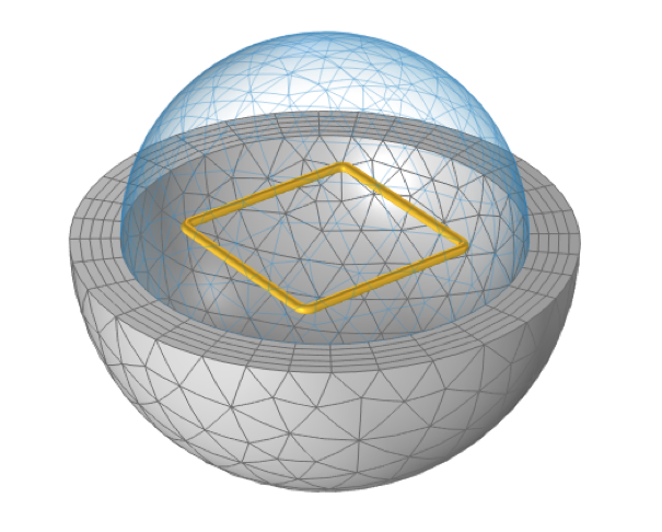
A square loop of wire, sitting within a spherical free space domain that is truncated by Infinite Element domains, has a defined total inductance.
This model uses a spherical domain truncated by Infinite Elements. The overall modeling approach is very similar to the Application Gallery example of a Helmholtz coil. This example uses both the Magnetic Fields, Currents Only interface and the Magnetic Fields interface, and demonstrates that these formulations will give identical results.
Although both the Magnetic Fields, Currents Only and the Magnetic Fields interfaces can be used, there are many differences between these two formulations. For now, we will focus on just three things that set the Magnetic Fields, Currents Only interface apart:
- It requires that there are no magnetically permeable materials, such as inductor cores, present.
- It requires that all conductors be modeled as having volume.
- It can compute not just total inductance, but also partial inductances.
Our model of an air-core loop of round wire clearly satisfies the first two requirements, so let’s focus on the third point: the computation of partial inductances.
While the concept of total inductance always requires a complete loop of current, the idea behind partial inductance is to subdivide the total loop into multiple parts, each of which contribute partial self-inductances and partial mutual inductances. The superposition of these contributions yields the total inductance of the closed loop. From both a theoretical and a modeling point of view, we have complete freedom in how to choose this subdivision, and can do whatever best suits our engineering purposes.
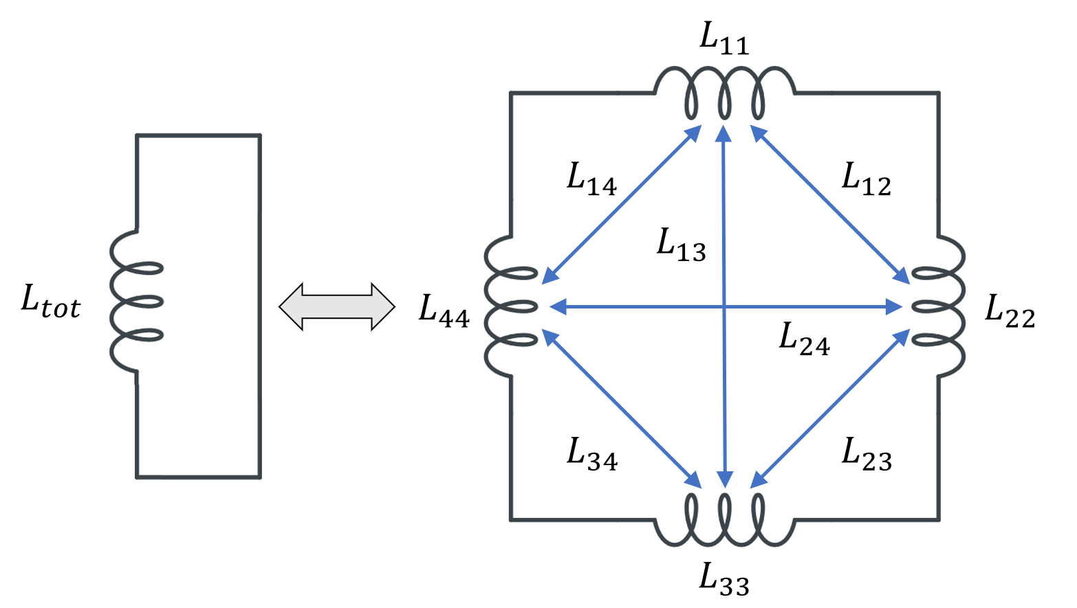
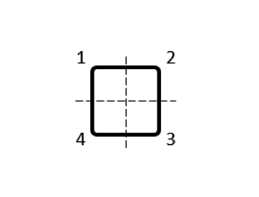
Subdividing a single inductor into 4 parts, with 4 partial self-inductances and 12 partial mutual inductances. For symmetry reasons, only 6 of the latter are named.
Several different possibilities for subdividing the conductor volume are shown in the table below. As for the modeling, for each of these domains we use a separate Conductor feature, with Terminal and Ground boundary conditions at either end of each domain, selected such that current always flows in the same direction around the loop. The output that we get is now a matrix of partial inductances, and it’s worth looking at the numerical values of this matrix. We refer to the terms on the matrix diagonal as the partial self-inductances and the off-diagonal terms as the partial mutual inductances.
| Coil Subdivision | Partial Inductance Matrix (nH) |
|---|---|
|
\begin{bmatrix}11.84 & 0.85 & -0.89 & 0.85\\0.85 & 11.84 & 0.85 & -0.89\\-0.89 & 0.85 & 11.84 & 0.85\\0.85 & -0.89 & 0.85 & 11.84\\\end{bmatrix} |
|
\begin{bmatrix}14.0 & 0.2 & -1.75 & 0.2\\0.2 & 14.0 & 0.2 & -1.75\\-1.75 & 0.2 & 14.0 & 0.2\\0.2 & -1.75 & 2& 14.0\\\end{bmatrix} |
|
\begin{bmatrix}25.38 & -0.08 \\-0.08 & 25.38 \\\end{bmatrix} |
|
\begin{bmatrix}38.4 & -1.3 \\-1.3 & 14.8 \\\end{bmatrix} |
|
\begin{bmatrix}49.3 & 0.5 \\0.5 & 0.3 \\\end{bmatrix} |
Table of partial inductance matrices for different choices of coil subdivision. The sum of the matrix terms is always the same.
Note that the partial self-inductances are always positive and, in this case, are much larger than any of the partial mutual inductances, which can be either positive or negative. The grand sum of all of the matrix terms equals that total inductance: L^{tot} = \sum_{i,j}L_{ij}. This holds, regardless of how the coil is subdivided. However, for different choices of subdivision, the matrix of partial inductances can become more heavily dominated by the self-inductances.
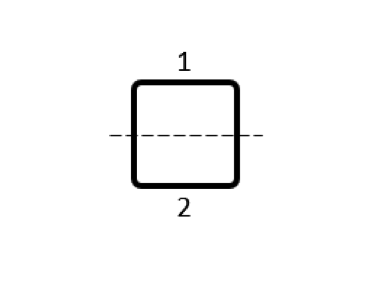
Based on this observation — that certain subdivisions of the coil lead to a more diagonally dominant partial inductance matrix — we are justified in building a submodel of just one section of the coil in free space, as shown in the figure below, and corresponding to the first subdivision in the table above. This model uses a single Conductor domain, with Terminal and Ground conditions on either end, and this model outputs just a single quantity: a partial self-inductance of 11.84 nH. This equals the diagonal terms of the previously computed partial inductance matrix.
A model of one-quarter of a square loop can compute the partial self-inductance, which gives a good prediction of the total inductance in this case. The Magnetic Fields, Currents Only interface allows for coils that terminate in free space, with Terminal and Ground conditions at the ends.
Now, this model seems to be creating and destroying current at the ends of the wire (where the Terminal and Ground boundary conditions are applied) but this is the distinguishing capability of the Magnetic Fields, Currents Only interface: It is capable of computing the partial self-inductance (and the partial mutual inductances) of any set of conductive domains, even those that are not connected in a closed loop.
For our next example, let’s consider the second subdivision of the coil. For this subdivision, we can look at just a short, straight, section of round wire — a particularly interesting case since there are handbook solutions — presented in the table below. In this case, we will look at the inductance and AC resistance over a frequency range, going from low frequencies, where the skin depth is much larger than the diameter, to high frequencies, where the skin depth is much smaller. To account for this, we have to use boundary layer meshing to resolve the skin effect. In addition, we omit the use of the Infinite Element domain, and use the default Exterior Boundaries condition on the boundaries of the spherical modeling space. This condition applies an approximate boundary condition based on the current flow within the model, so the radius of the computational domain does need to be studied.
| Handbook Values for AC Inductance and Resistance of a Round Wire | |
|---|---|
| Low-Frequency Inductance | \frac{\mu_0}{2\pi}\ell\left[ \ln\left( \frac{2\ell}{r}\right) -\frac{3}{4}\right] |
| High-Frequency Inductance | \frac{\mu_0}{2\pi}\ell\left[ \ln\left( \frac{2\ell}{r}\right) -1\right] |
| DC Resistance | \frac{\ell}{\sigma \pi r^2} |
| AC Resistance | \frac{\ell}{\sigma \pi (2r\delta – \delta^2)} |
| Length: \ell, Radius: r, Electric Conductivity: \sigma, Skin Depth: \delta =\sqrt{ \frac{2}{\omega \mu_0\sigma}} | |
The computed results show exact agreement for the DC resistance and close agreement (within 1%) for the low-frequency inductance. The slight disagreement for the low frequency has to do with end effects; the agreement between a numerical model and handbook value for a straight wire becomes better the longer a length of wire is analyzed.
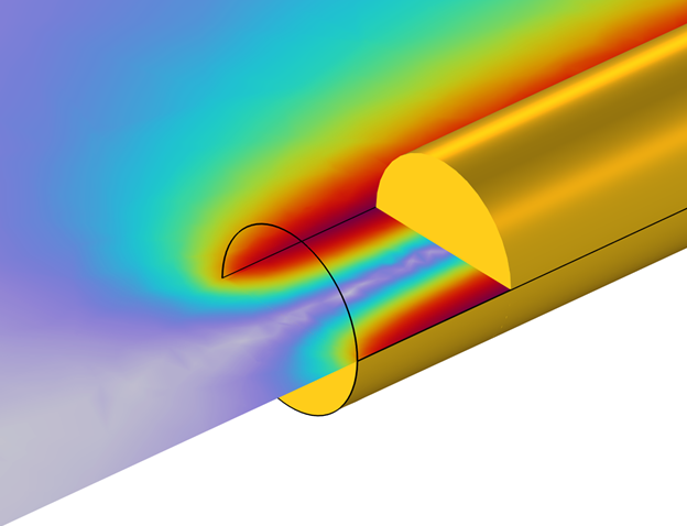
Cutaway closeup view of the wire interior. The computed magnetic field shows an end effect.
The AC resistance also shows good agreement over a wide range, but there is a noticeable deviation at higher frequencies, where the skin depth is much smaller than the wire diameter. This deviation is due to a different issue: At such high frequencies, we would need a very fine boundary layer mesh to resolve the skin effect.
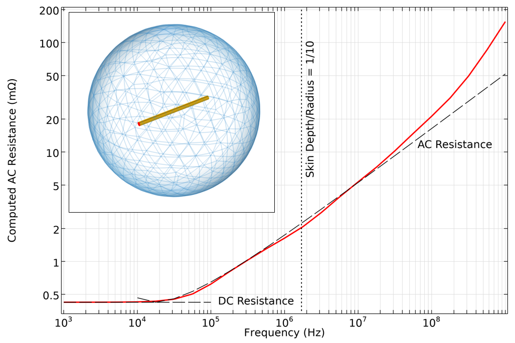
Computed AC resistance of a straight wire, as compared to handbook equations based on skin depth. At very high frequencies, a very fine mesh would be needed, and the assumption of negligible displacement currents no longer holds.
At these higher frequencies there is yet another issue: The assumption that nearby dielectrics can be ignored is no longer valid. In other words, the displacement currents start to become significant. In this regime, we should instead use the Magnetic Fields formulation, which can model the currents as flowing on the surfaces of the conductors, rather than solving for the fields within the volume. The Magnetic Fields interface solves for displacement currents as well as conductive and inductive currents. The Magnetic Fields, Currents Only interface neglects all displacement currents and only considers conductive and inductive currents within the conductor domains themselves.
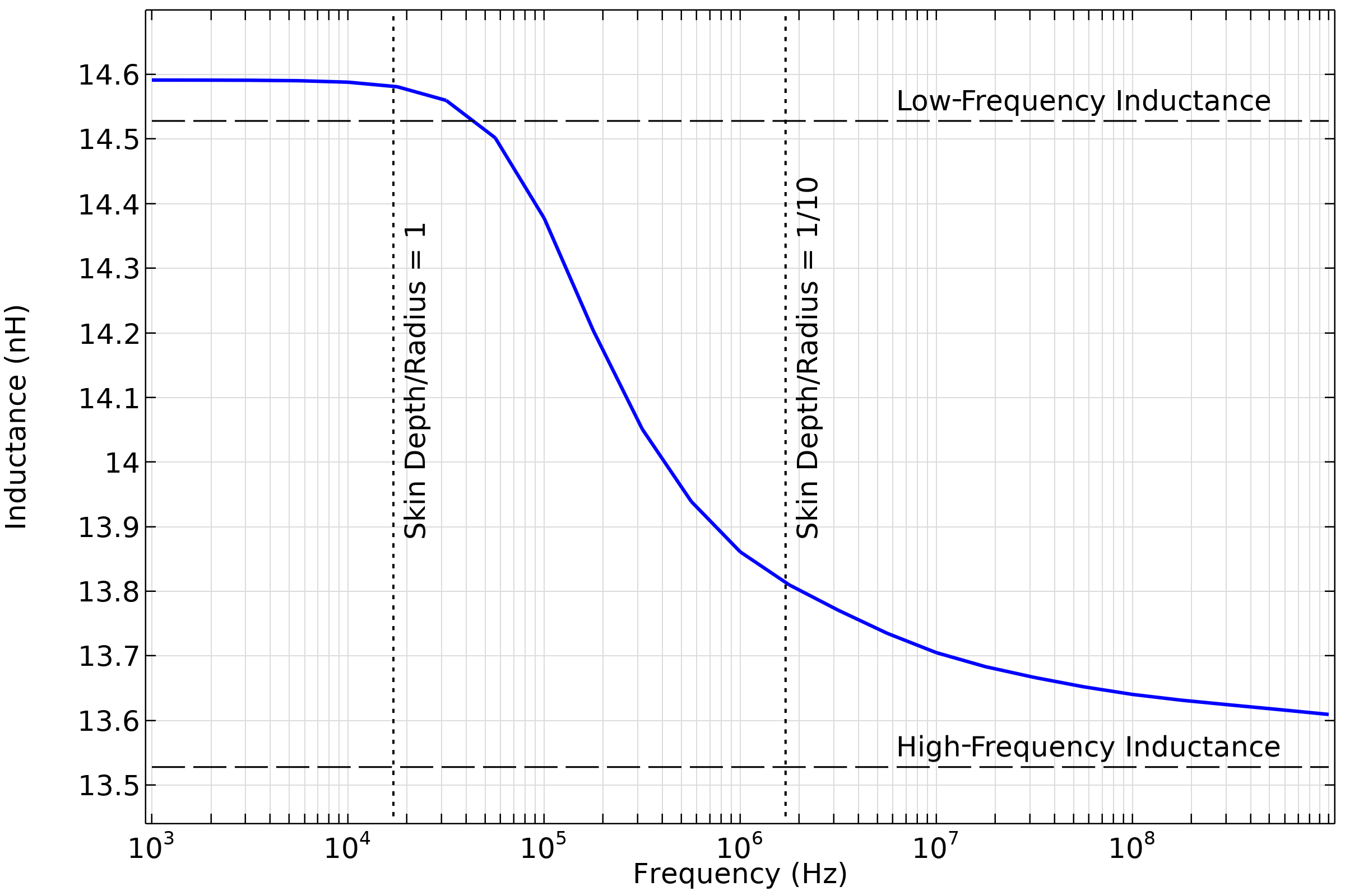
Computed partial self-inductance of a straight wire, compared to low- and high-frequency handbook solutions that neglect end effects.
So, now that we understand how to compute partial inductance, and the regime of applicability of this formulation, how can we use this interface with confidence? It is important to note that we can never measure any of these partial inductances, as only the total inductance of a closed loop is measurable. But, supposing that we have a large system with a lot of complexity, then we are likely in a situation where computing the total inductance is quite expensive.
In a case where we are only interested in redesigning one small subsystem, we make two assumptions:
- The partial mutual inductances between the modeled and nonmodeled components have a relatively small effect on the total inductance.
- The partial self-inductance of the components that are not being modeled stays relatively fixed.
If these assumptions hold true, then it is reasonable to only model that one part (or just a few parts) of a system. Although we might not ever want to compute the total inductance, there can still be predictive value in this submodel as long as the above assumptions — and the concept of these partial inductances being contributions to the total inductance — are understood.
Now, let’s look at a few typical examples of the applicability of this interface.
Typical Applications of the Magnetic Fields, Currents Only Interface
Situations where the Magnetic Fields, Currents Only interface will be useful include:
- Computing partial inductances of circuit board components
- Power bus systems
- Cabling and connectors
- Insulated-gate bipolar transistors (IGBTs)
- Coils in the absence of nearby magnetic materials
One example is a circuit board with several air-core inductors, as shown below. With the knowledge we have accrued, we can now confidently build models that extract the partial self-inductance of a single inductor, or the partial self-inductances and partial mutual inductances between several closely spaced inductors. For a related example to start with, see Inductance Matrix Calculation of PCB Coils.
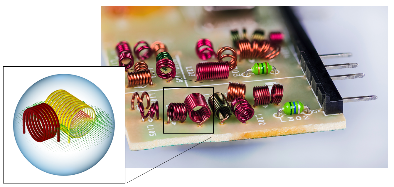
An electrical component that contains many air-core inductors. It is possible to compute the AC resistances and the partial inductance matrices at just a few of these inductors at a time by using the Magnetic Fields, Currents Only interface.
Closing Remarks
Here, we have introduced the use of the Magnetic Fields, Currents Only interface for computing total and partial inductances and AC resistances. By starting with a case that we can verify against other approaches, we verify the overall correctness of the total inductance calculation. We then looked at partial inductance and how the partial and total inductance are related. We also looked at computing the AC resistance, which helped us understand the regime of validity of the Magnetic Fields, Currents Only interface for frequency-domain modeling. With this information, we are now ready to tackle these types of problems with confidence!
You can learn about the AC/DC Module here or contact us for more details.


Comments (3)
Marco Antolovic
November 7, 2022Hi Walter,
Thanks for the explanation on partial inductance. Is it possible to have the model you presented above (Quarter of square loop and straight conductor)?
Thanks,
Marco
Walter Frei
November 7, 2022 COMSOL EmployeeHello Marco,
This blog is more about the conceptual points. For the purposes of learning the Magnetic Fields, Currents Only interface, please refer to these tutorial examples:
https://www.comsol.com/model/magnetic-field-of-a-helmholtz-coil-15
https://www.comsol.com/model/inductance-matrix-calculation-of-pcb-coils-89921
What we’ve presented here is really more of a geometric variation on the modeling approach shown in the above.
Happy Modeling!
Poonam Chand
June 26, 2024Hi Walter,
Thanks for such a valuable information. Can you please tell me if we can compute the Partial Inductance of any coil using Partial Element Equivalent circuit method (PEEC) using AC/DC module? In PEEC, we can leave the discretization of the air making the simulation time faster.
more about PEEC: https://en.wikipedia.org/wiki/Partial_element_equivalent_circuit