
Convolution is a useful mathematical operation, applied in various fields for signal and image processing, statistics, and so on. Acoustic engineers often use convolution to process acoustic signals in order to extract the desired information or better interpret sound. In this blog post, we introduce three methods for performing convolution in the COMSOL Multiphysics® software. We will discuss implementing convolution by applying the methods to the low-pass filtering of a room impulse response (IR) and show one example of the auralization of room acoustics.
Convolution: Definition and Methods
Physically, convolution gives you the information on the amount of overlap between two signals that are represented in the time domain, the frequency domain, or the spatial domain. For time-domain signals, it’s mathematically defined as
Here, t and \tau are the time variable and dummy variable used for time integration, respectively, and \ast represents the convolution operator.
At each t, the equation calculates the time integral of the product of one function, f(\tau), in its original form with the other function, g(t-\tau), that is reflected and shifted by t. The operation is commutative, i.e., the result stays the same no matter which function is reflected and shifted. The integral should be conducted for all values of shift (t), giving the convolution result as a function of t.
This integral form, called convolution integral here, is suited for processing smooth and continuous functions. For discrete data, such as digitized sound signals, this method requires a highly demanding numerical integration scheme, which often results in a heavy computational load. To avoid this, the following discrete convolution can be used for processing discrete signals:
Here, \Delta t is the sampling interval.
By approximating the integral to a summation of discrete samples, the discrete convolution can be computed faster than the convolution integral.
When the Fourier transform of the two signals exists, the discrete convolution can be evaluated more efficiently using the fast Fourier transform (FFT) based on the convolution theorem:
Here, \mathcal{F} and \mathcal{F}^{-1} are the Fourier and inverse Fourier transformation operators, respectively. The convolution theorem uses the fact that the Fourier transform of the convolution of two functions in the time domain is equivalent to the product of the Fourier transforms of the signals (the signals in the frequency domain). Modern real-time convolution technology generally uses the FFT because of its excellent efficiency.
Low-Pass Filtering of Room Impulse Response
Here, we will demonstrate how to implement convolution using the convolution integral, the discrete convolution, and the convolution theorem in COMSOL Multiphysics®. We will go over the essential steps of these methods via an example where we apply low-pass filtering to an impulse response (IR) obtained from the Small Concert Hall Acoustics tutorial model. (Low-pass filtering is widely used to extract only the lower bass tones in sound designs.) This IR data is loaded and stored in an interpolation function (Interpolation 1, in this case). A plot of the data is shown below.
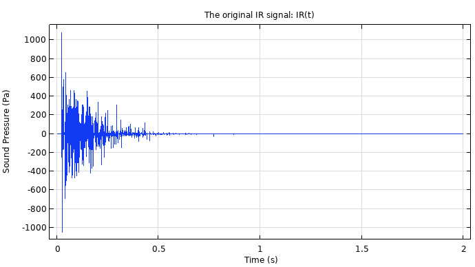
A plot of the room IR.
The duration and the sampling frequency of the data are 2 s and 44,100 Hz, respectively.
As for the low-pass filter, we use the 4th-order Butterworth filter. The transfer function of the filter, TF(f), is defined as follows:
with
where f and \omega represent the frequency and angular frequency, respectively. \omega_c is the angular frequency at the cutoff frequency. \Pi is the product operator representing the product of a sequence.
In the example, the 4th-order filter with a cutoff frequency of 2 kHz is defined with an Analytic function (in this case, Analytic 1). The images below show how the function is defined, the frequency response of the function in respect to its real and imaginary component, and the gain characteristics of the filter defined by such a function.
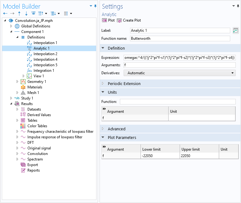
The transfer function of the 4th-order Butterworth filter is defined using an Analytic function.
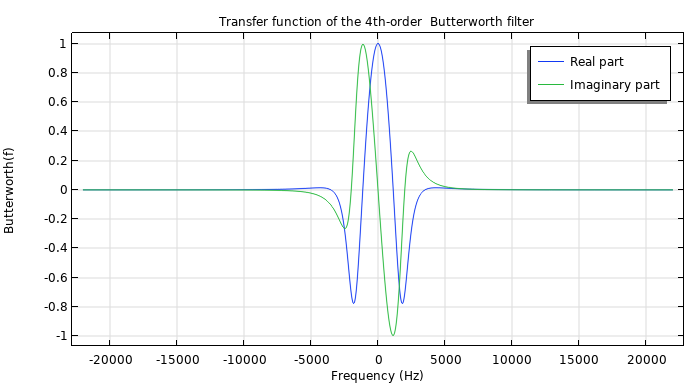
The frequency response of the transfer function in respect to its real and imaginary component.
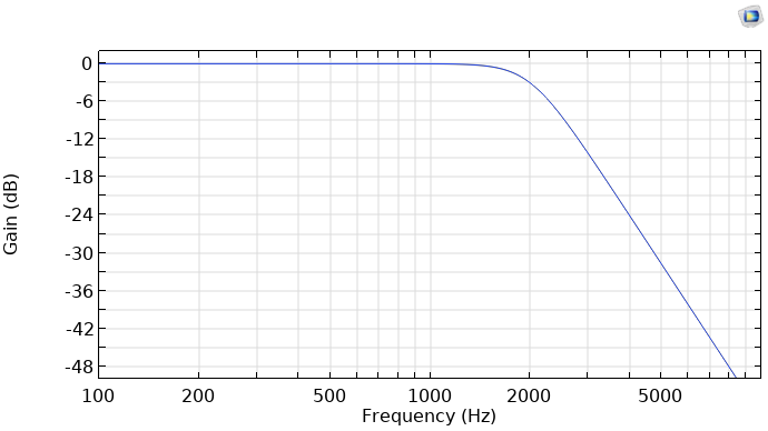
The gain characteristic of the low-pass filter.
The gain characteristic indicates that the low-pass filter has a flat passband up to the cutoff frequency of 2 kHz (at which point the filter attenuates the input power by half or 3 dB). Above the cutoff frequency, the filter gain decreases at a rate of -24 dB per octave.
Let’s now go over the three methods for performing convolution in COMSOL Multiphysics®.
Method 1: Direct Treatment of Convolution Integral
We start with the direct treatment of the convolution integral. Here, you need two time-domain signals for input. For the first signal, the room IR, it has already been defined as Interpolation 1. The second signal, the low-pass filter, is defined in the frequency domain. We need to convert it to the time domain by taking an inverse discrete Fourier transformation (IDFT) of the signal. This is done via the following steps.
Step 1
Create a Grid 1D dataset and name it Grid 1D_f. This generates a frequency grid specified in a frequency range (-22050 Hz, 22050 Hz) that corresponds to the frequency spectrum of the room IR data. It will be used in plotting the signals in the frequency domain.
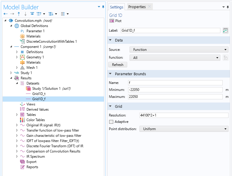
Setting for the Grid 1D_f dataset.
Step 2
Perform IDFT of the low-pass filter using a Function plot in the 1D Plot Group feature with the Grid 1D_f dataset. In the Output section of the Settings window, select Discrete Fourier transform from the Display list, select Real part from the Show list, and check Inverse transform.
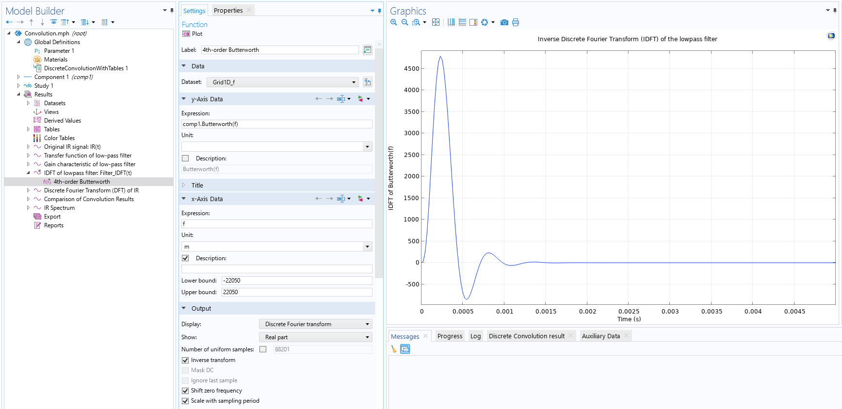
The settings and plot of the IDFT of the low-pass filter.
Step 3
Add plot data to Table 1.
Step 4
Define an interpolation function (Interpolation 2) with the data stored in Table 1.
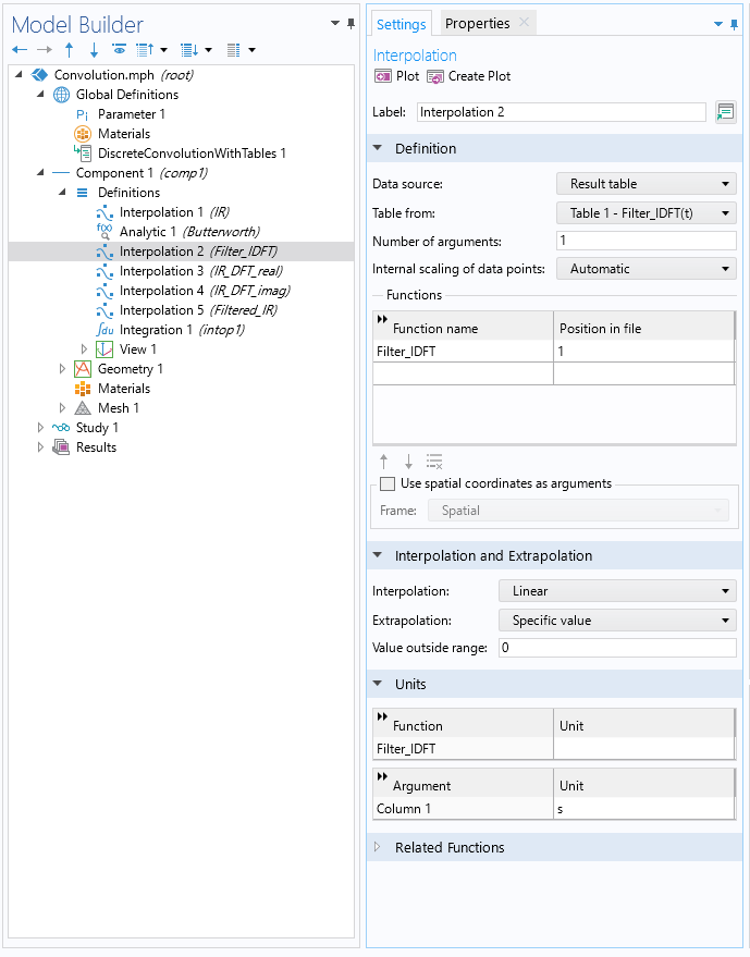
The setting of Interpolation 2.
Now we have two time-domain signals that are ready for convolution. Although an infinite time interval, -\infty, \infty, is assumed in the definition, the integral only needs to be calculated in a finite time interval of 0–2 s since both input signals are set to zero outside of that time range. The procedure for the convolution integral is shown below.
Step 1
Define an interval in the Geometry node so that its start and end values correspond to the integral interval (0–2 s).
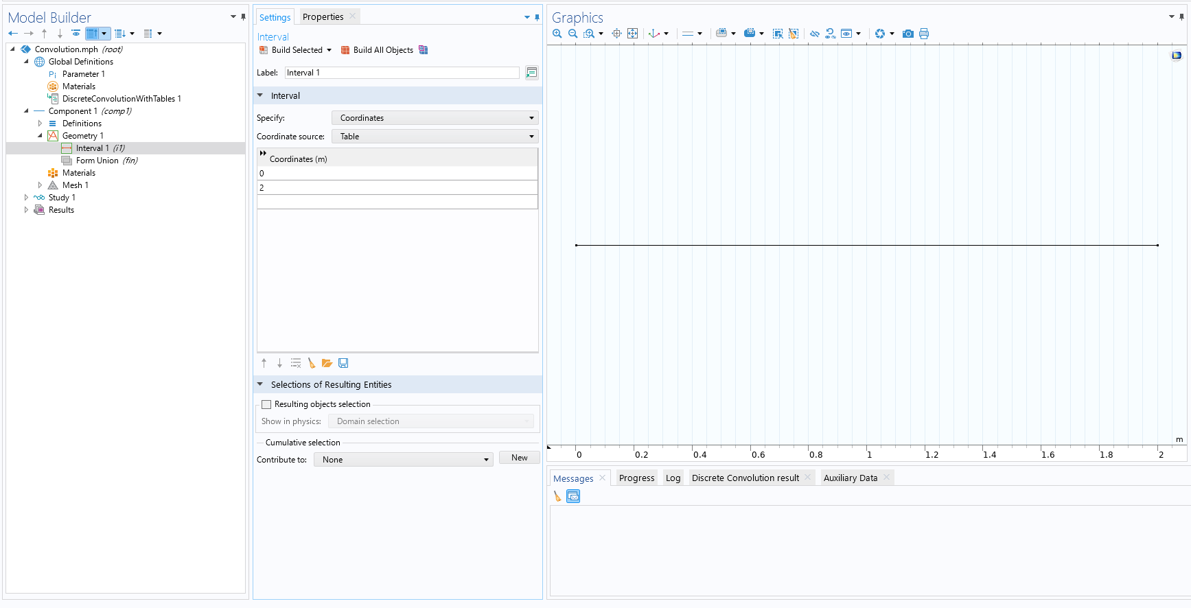
Create the interval.
Step 2
Define the integration operator intop1 on the interval.
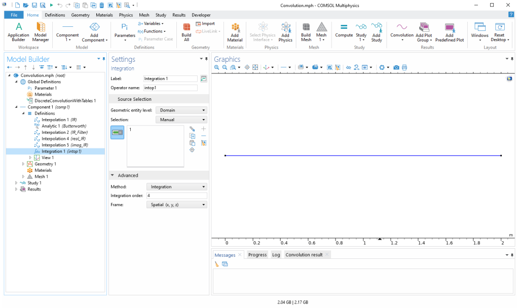
Definition of the integral operator.
Step 3
Discretize the interval with a uniform line mesh whose size equals the sampling interval of the original room IR data.
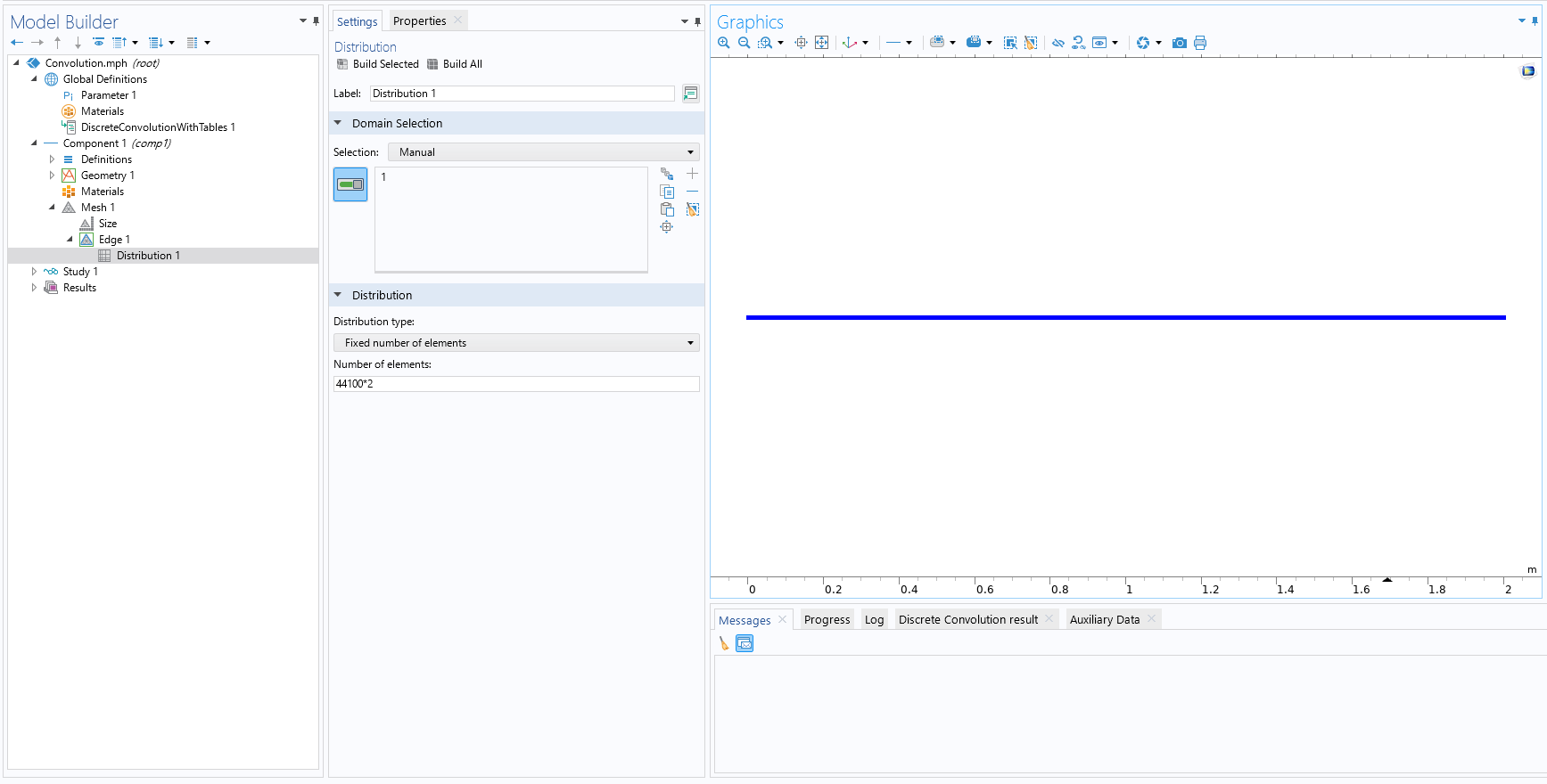
Discretization of the interval.
Step 4
Run a Stationary study so that the interpolation functions and the intop1 operator can be used in the Results section.
Step 5
Create a Grid 1D dataset and name it Grid 1D_t. This generates a time grid for defining the time signal in a range of 0–2 s, with a sampling frequency of 44,100 Hz.
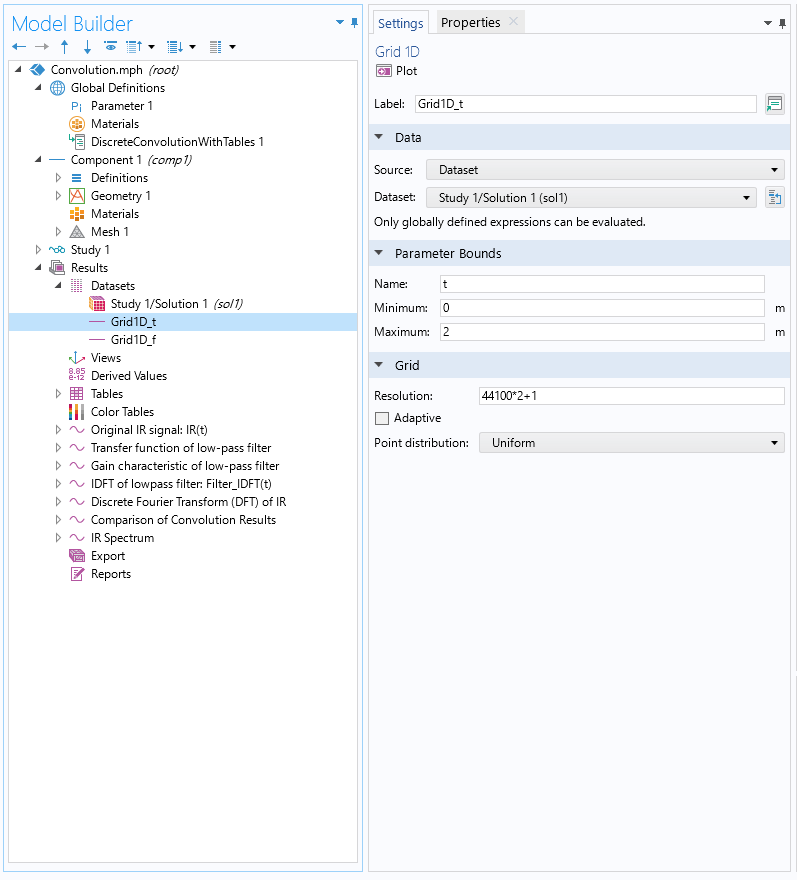
Settings for the Grid 1D_t dataset.
Step 6
Carry out the convolution integral in a 1D plot using Grid 1D_t as the source dataset.
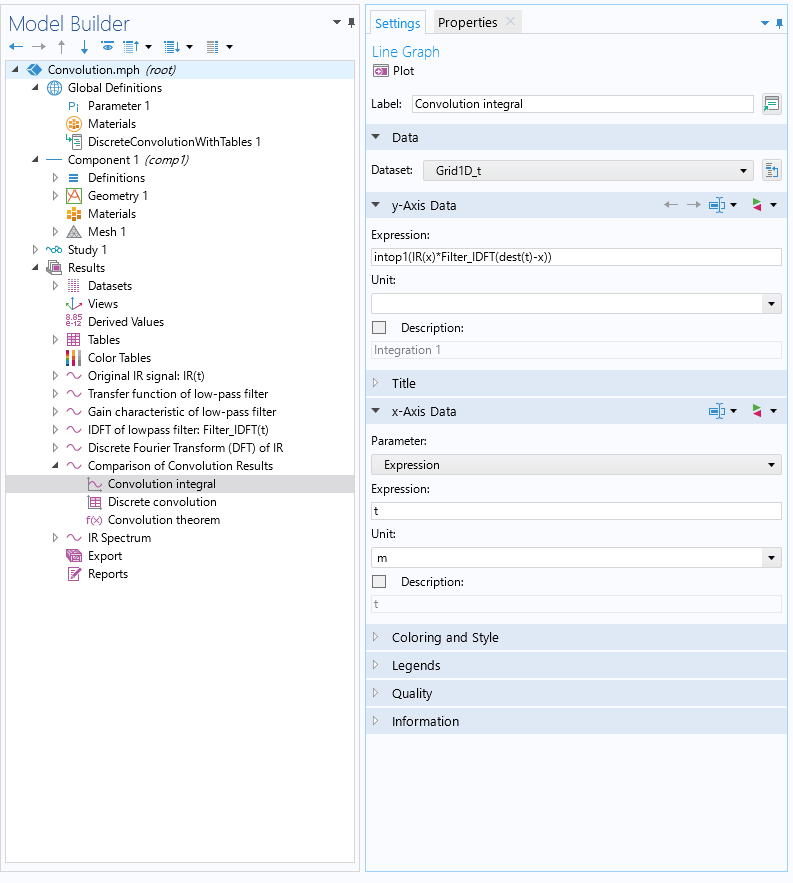
Expression for the convolution integral using the dest operator.
Here, IR and Filter_IDFT are the interpolation functions of the room IR and the low-pass filter IR defined in Interpolation 1 and Interpolation 2.
Note that the dest operator enforces the evaluation of the function on the destination point instead of the source point.
Method 2: Standard Discrete Convolution
Discrete convolution is well used in practice. To perform discrete convolution in COMSOL Multiphysics®, the use of the Application Builder is essential. With the Method Editor in the Application Builder, you can use Java® code to create methods that you can run to automate or extend operations in the model tree. This blog post exemplifies the method for performing convolution with table-stored data.
The following image shows the implemented code and the settings, and the following table presents the variables defined in the code.
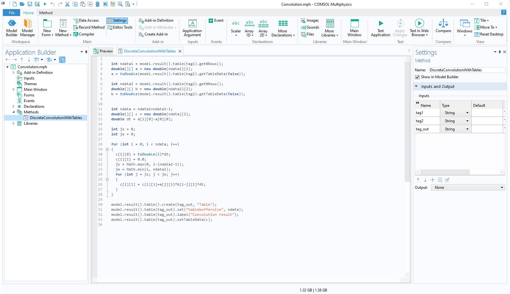
Java method performing the discrete convolution with stored data in tables.
| Name | Type | Description |
|---|---|---|
| a | Double (array 2D) | Data from the first input table |
| b | Double (array 2D) | Data from the second input table |
| c | Double (array 2D) | Convolution result |
| ndata1 | Integer (scalar) | Length of a |
| ndata2 | Integer (scalar) | Length of b |
| ndata | Integer (scalar) | Length of c |
| dt | Double (scalar) | Sampling interval |
| js | Integer (scalar) | Start value of the summation index |
| je | Integer (scalar) | End value of the summation index |
Variables defined in the Java® program.
The code performs the discrete convolution with the data stored in two input tables and exports the result to an output table. The following notes can be used to better understand the code:
- 2nd–4th lines: extract the data and the length of the data from the first input table
- 6th–8th lines: extract the data and the length of the data from the second input table
- 11th–13th lines: define the length of the result, create the double precision array that stores the convolution result, and define the sampling interval
- 18th–28th lines: perform the for loop to start the discrete convolution, from the first time step to the last
- 30th–33rd lines: export the result to the output table labeled Discrete convolution result
Note that the length of the result data is the sum of the two input tables’ length minus 1, and the start value (js) and end value (je) of the summation index are defined so that js is smaller than the length of the second table and je is smaller than the length of the first table (see 22nd and 23rd lines in the code, respectively).
To run the program, the plot of two time signals must be stored in tables. The plot data of the IDFT of the low-pass filter is stored in Table 1. For the room IR, you need to create a function plot of the room IR in the 1D Plot Group feature with the Grid 1D_t dataset and copy the plot data to Table 2.
The tag names of the tables can be entered in the Settings window of a Method Call feature that is added to the model tree. After all settings are set up, you can perform the discrete convolution by clicking the Run button in the Method Call Settings window.
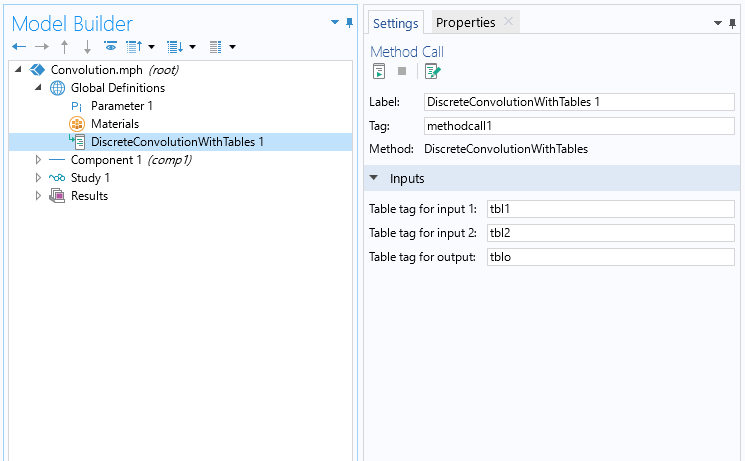
Inputting table tags in the Settings window for the Method Call feature.
Method 3: Discrete Convolution Based on the Convolution Theorem
The last method performs the convolution based on the convolution theorem, i.e., the use of the DFT. In this case, the DFT of the room IR and the transfer function of the low-pass filter are used. The method is as follows:
Step 1
Plot both the real and imaginary parts of the DFT of the room IR in two Function plots (one for each) within the same 1D plot group. In the settings, choose Discrete Fourier transform from the Display list. Then, select Real part or Imaginary part from the Show list, respectively for plotting the real and imaginary parts of the DFT of the room IR. The check boxes are default settings.
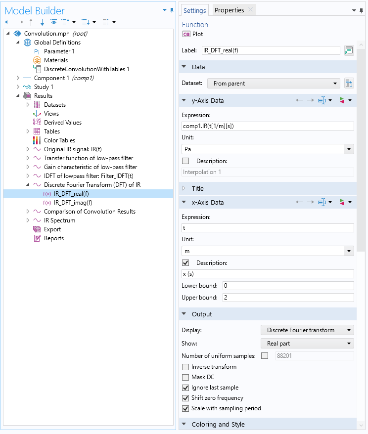
DFT of the room IR in a 1D plot.
Step 2
Copy the plot data of real and imaginary parts of the DFT of the room IR to Table 3 and Table 4, respectively.
Step 3
Define Interpolation 3 and Interpolation 4 with stored data in Table 3 and Table 4, respectively.
Step 4
Perform the convolution by calculating the IDFT of the pointwise product of the DFT of the room IR and the low-pass filter. The pointwise multiplication and IDFT are both done in a single Function plot using the Grid 1D_f dataset.
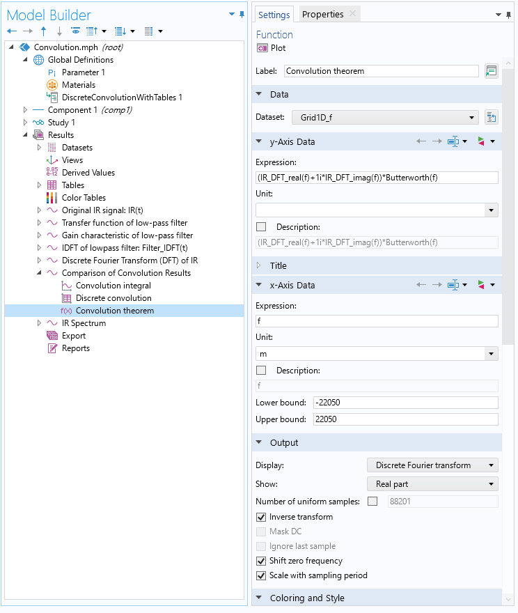
The IDFT of the product of the DFT of the room IR and the low-pass filter. The Inverse transform check box in the Settings window is selected to perform the inverse transformation.
Here, real_IR and imag_IR are the real part and the imaginary part of the DFT of the room IR and are defined in Interpolation 3 and Interpolation 4, respectively. Butterworth is the transfer function of the low-pass filter defined in Analytic 1.
Note that the convolution theorem method performs the circular convolution, meaning if the length of the grid’s interval is insufficient, a circular overlap arises.
Result of Low-Pass Filtering
The graphs below show the low-pass filtered room IR calculated by the three methods, and you can see good agreement among the three methods.
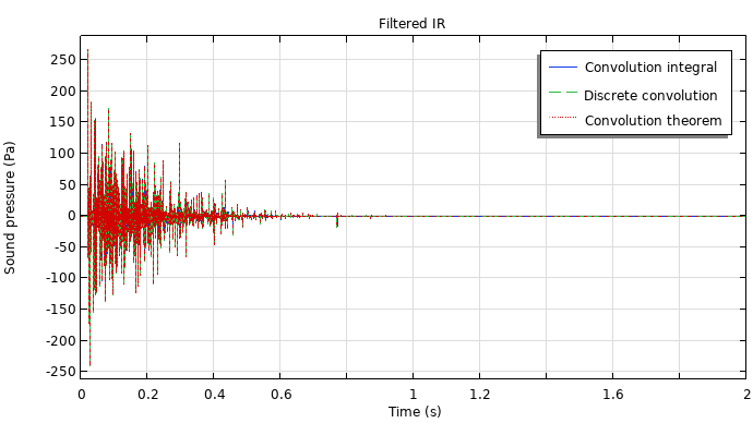
A comparison of the convolution results calculated by the convolution integral, the discrete convolution, and the convolution theorem.
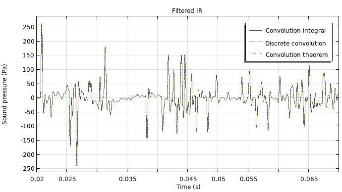
The convolution results in the range of 0.02–0.07 s.
The next figure presents a comparison of the spectra of the room IR before and after filtering. You can confirm that the filtered spectrum decreases above 2 kHz, which is the cutoff frequency of the low-pass filter. This result supports success of the convolution implementation.
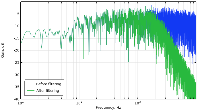
Spectra of the room impulse response before and after filtering.
Application to Auralization
Let’s move on to the example of auralization. This example covers the convolution of the room IR and an audio recording captured in an anechoic chamber. Under the assumption of a linear time-invariant system, a response from an arbitrary input can be assessed by convolution of IR and input signal. Based on this theory, acousticians evaluate sound fields auditorily by the convolution of IR simulated using computational methods and anechoic sound. This simulation process is called auralization, which spans from the creation of sound data to hearing it. The example model (accessed via the button in the next section) performs the auralization of a trumpet sound in the small concert hall model using the standard discrete convolution method described earlier. You can also export the convolution result as a WAV audio file for playing in an audio or media player. In the following, you can compare the anechoic and the reverbed trumpet sounds.
The trumpet as it sounds when played in an anechoic chamber.
The trumpet as it sounds when played in the small concert hall, using auralization.
The above example is a monaural sound, which is different from a binaural sound we usually hear. However, we can generate more realistic sounds by combining the head-related transfer function or the sound field reproduction techniques such as an Ambisonics (see, for example, Ref. 1). Such examples will be demonstrated in the future blog topic.
Next Steps
Further explore the model discussed in this blog post by clicking the button below, which will take you to the Application Gallery.
Further Reading
Learn more about data processing in acoustics modeling from the following blog posts:
- Computing Transient Sound Pressure Levels in COMSOL®
- Modeling Room Acoustics Using a Hybrid Approach
References
- M. Vorländer, Auralization: Fundamentals of Acoustics, Modelling, Simulation, Algorithms and Acoustic Virtual Reality, Springer Science & Business Media: Berlin/Heidelberg, 2007.
The anechoic sound is provided by The Open AIR Library under CC BY 4.0.
Oracle and Java are registered trademarks of Oracle and/or its affiliates.


Comments (0)