How to Model Sparging in COMSOL Multiphysics®

Sparging, a mass transfer process between a gas and a liquid, is commonly encountered in industrial applications such as beverage carbonation and photobioreactors, or even at home for aeration in aquariums. In this blog post, we detail how to model a type of sparging, carbonation, using the COMSOL Multiphysics® software.

What Is Sparging?

Sparging is the process of bubbling a gas into a liquid to either dissolve it in the liquid or to strip the liquid off of some dissolved components. As mentioned above, the process entails mass transfer from a gas into a liquid or vice versa. One example of sparging is the process of oxygen stripping, in which nitrogen is bubbled through a liquid to push out or remove oxygen and other dissolved gases. Another example is dissolution, where a gas is dissolved into a liquid. The dissolved species can further react with the other components in the liquid, altering the liquid’s chemical composition. Carbonation and aeration are common examples of such sparging/dissolution.

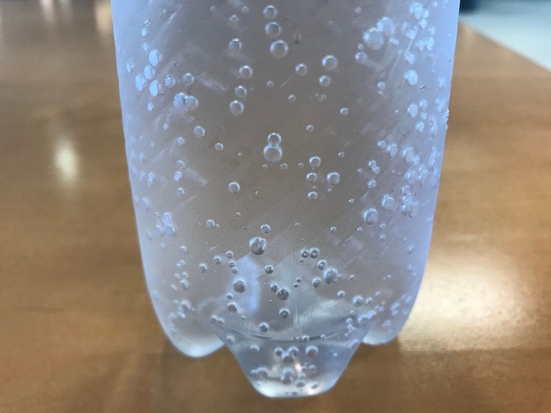
Bubbles from carbonation in a bottle of sparkling water.

When we open a bottle of soda, sparkling water, or any carbonated beverage, we experience a “fizz” due to a pressure release accompanied by buoyancy, leading to the rise of carbon dioxide bubbles. Before we open the bottle, however, carbon dioxide is dissolved into the beverage (CO₂ (aq)). This dissolution is achieved by passing carbon dioxide bubbles (usually at high pressures for supersaturation) through the beverage. When the carbon dioxide bubbles pass through the beverage, there is mass transfer from the gas to the liquid across the surface of the bubbles and the dissolved carbon dioxide reacts with water to form carbonic acid. This entire process is known as carbonation.

In this blog post, we will take a look at how to model the carbonation process via the dissolution of carbon dioxide in water. In other words, we will make virtual carbonated water.

A Closer Look at Carbonation

Consider a glass of water into which carbon dioxide is introduced from its base, as shown in the schematic below. The carbon dioxide bubbles rise due to buoyancy and move through water, transferring mass and momentum and finally exiting through the top surface. Note that the dissolved carbon dioxide reacts with water to produce carbonic acid. Therefore, in order to model and understand carbonation in this glass, we need to resolve:

• Mass and momentum transport of water and carbon dioxide bubbles; i.e., multiphase flow
• Mass transfer of carbon dioxide from bubbles to liquid; i.e., dissolution
• Mass transport of dissolved carbon dioxide and any subsequent reactions that take place (like the production of carbonic acid)

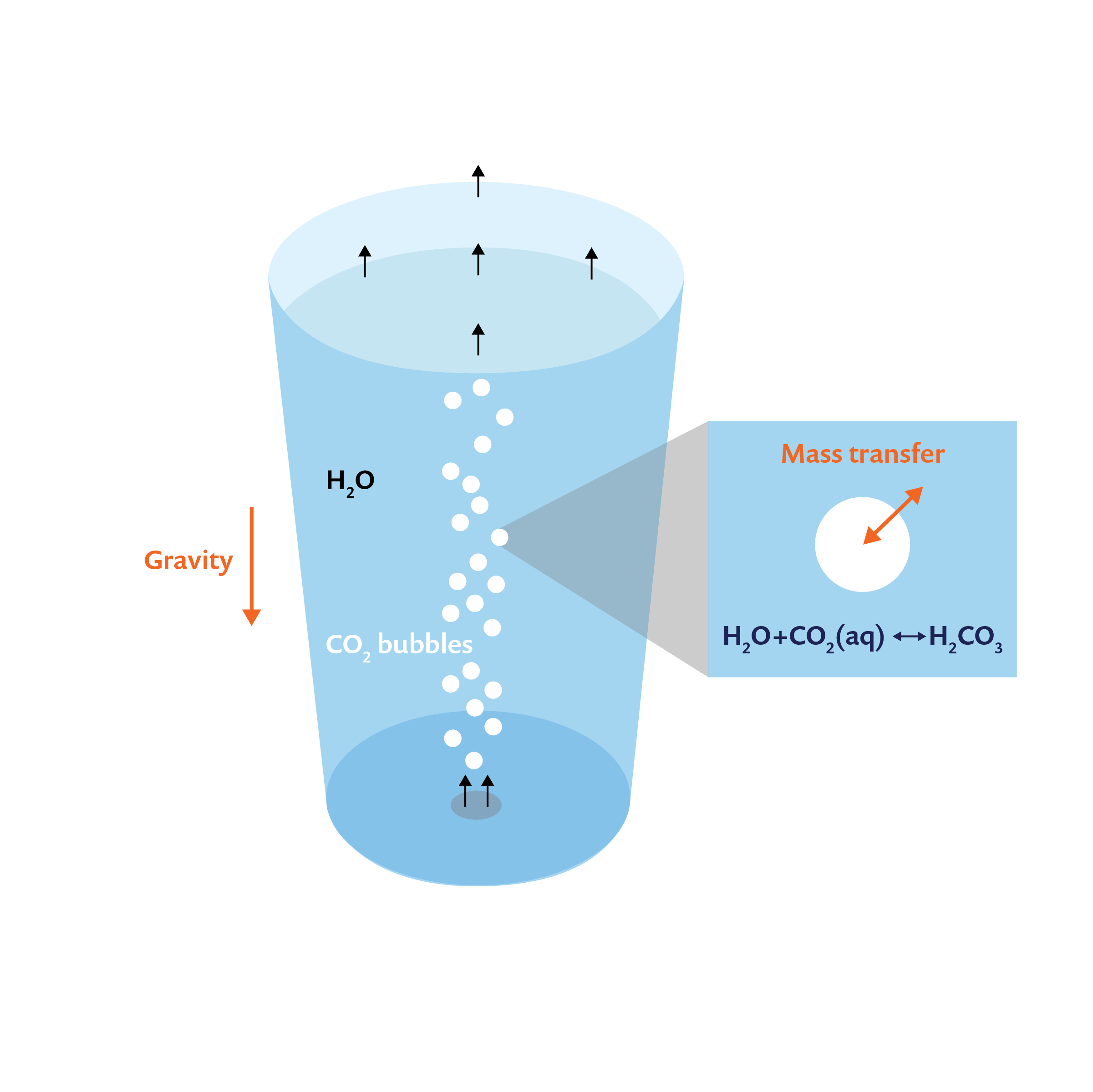
Schematic of carbonation in a glass of water, with carbon dioxide bubbles entering from the bottom.

Modeling Sparging in COMSOL Multiphysics®

Let’s take a look at the required interfaces and conditions in COMSOL Multiphysics to resolve the above-mentioned aspects of sparging. The problem, as depicted in the above schematic, is axisymmetric. Therefore, we can set up the model using a 2D axisymmetric component. In terms of modeling multiphase flow, we use the Bubbly Flow, Laminar Flow interface because the volume fraction of bubbles is less than 1% and the density of carbon dioxide gas is negligible compared to the water. When the volume fraction of bubbles is less than 1%, particle tracing can also be used to solve for the transport of bubbles. However, note that bubbly flow can be used to model systems where the bubble volume fraction is greater than 1% (around 10% or less).

In addition, laminar flow has been chosen because the Reynolds number, calculated based on the bubble velocity, is lower than 2000 for the internal flow.

Tip: Read a blog post on the different types of multiphase flow interfaces in the COMSOL® software, including their advantages, disadvantages, and the corresponding underlying assumptions.

The Bubbly Flow, Laminar Flow interface solves for velocity, pressure, and the effective gas density. It also allows for the computation of the number density of gas bubbles and the relevant interfacial area (when the Solve for interfacial area option is chosen in the settings). This enables the computation of mass transfer between the bubbles and liquid using two-film theory, which will be discussed later.

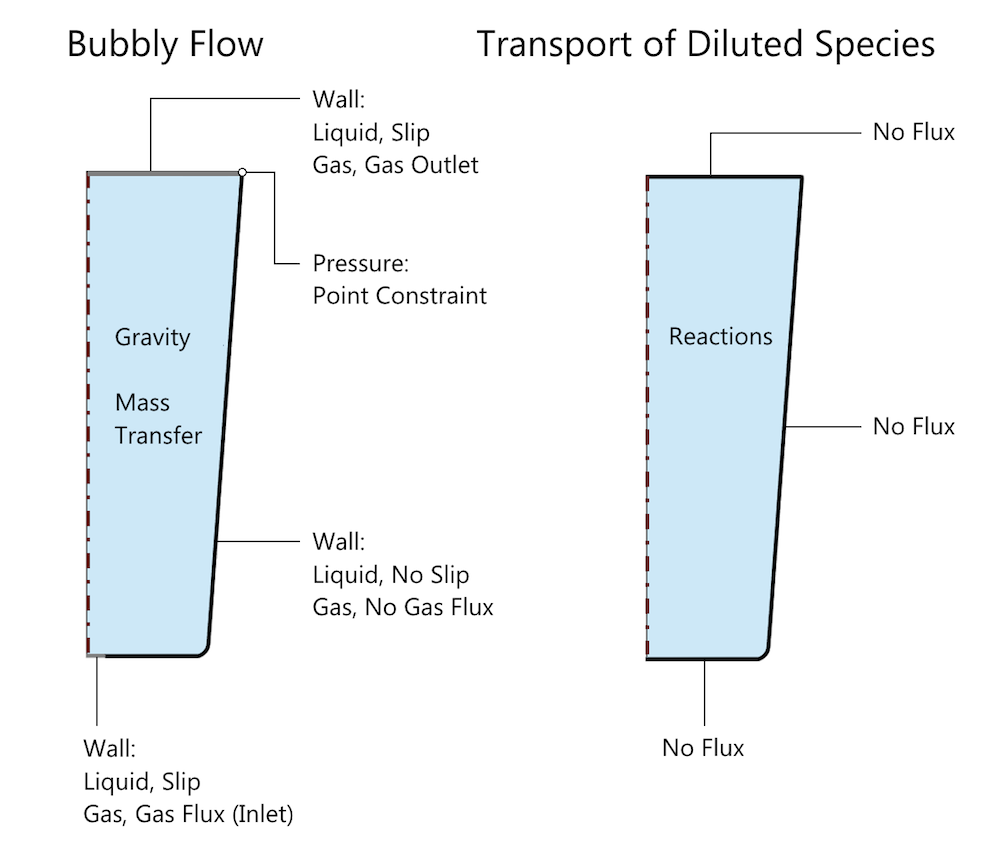
Schematic of the problem setup in COMSOL Multiphysics, with the relevant boundary and domain conditions for the Bubbly Flow and Transport of Diluted Species interfaces. Mass transfer of carbon dioxide is specified through a Reactions condition and the carbonic acid reaction is specified through an Equilibrium Reaction condition, both indicated by Reactions in this schematic. Note that the default domain conditions, such as Fluid Properties, Transport Properties, and Initial Values, are not indicated.

While modeling the fluid flow, note that we are assuming that the deformation of the free surface — i.e., the top surface of the water — is negligible. However, as this is a free surface, a Slip wall condition is chosen at the boundary, as shown in the figure above. This allows for the tangential motion of the water but restricts the normal velocity to zero. Gas inlet and outlet conditions are specified under the Wall boundary conditions in this interface. (More details about this process can be found in a previous blog post on modeling bubbly flow in a glass of beer.) The inlet gas flux is ramped from zero to the required value for consistency, a method of load ramping in time that is generally a good practice.

The transport of aqueous carbon dioxide and carbonic acid that results from the equilibrium reaction of carbon dioxide and water is modeled using the Transport of Diluted Species interface. This interface solves for the concentrations of aqueous carbon dioxide and carbonic acid. Note that we are only considering the reaction leading to the formation of carbonic acid in this case. The relevant boundary conditions for Bubbly Flow (bf) and Transport of Diluted Species (tds) are shown in the above figure.

The mass transfer of carbon dioxide from bubbles to liquid is modeled through a Mass Transfer condition in the Bubbly Flow interface. In this case, we use the Two-film theory option, which uses Henry’s law to compute the required mass transfer from gas to liquid, m_{gl}, given by:

where:

• k is the mass transfer coefficient that has to be specified, derived from experiments or literature
• c is the concentration of the solute; in this case, the concentration of aqueous carbon dioxide, c_CO2, that is computed through the Transport of Diluted Species interface
• M is the molecular weight of the gas (carbon dioxide)
• a is the interfacial area per volume, computed from the Bubbly Flow interface
• {c^*} is the equilibrium concentration given by Henry’s law (c^* = (p+p_{ref})/H), where:
  • p is the relative pressure computed from the Bubbly Flow interface
  • p_{ref} is the reference pressure specified under the Bubbly Flow interface
  • H is the Henry’s constant derived from experiments or literature

The mass transfer from gas to liquid is a source of aqueous carbon dioxide and is accounted for in the Transport of Diluted Species interface through the Reactions term, as shown below. In addition to the coupling between the Transport of Diluted Species and Bubbly Flow interfaces, the velocity of the liquid phase computed from the Bubbly Flow interface is passed under the Transport Properties domain settings of the Transport of Diluted Species interface. This accounts for the convective transport of aqueous carbon dioxide.

Settings of the Mass Transfer condition in the Bubbly Flow interface. All parameters specified in this domain feature are defined under the Parameters node, except for c_CO2, which is the concentration of carbon dioxide computed under the Transport of Diluted Species interface.

Settings for the Reactions term under the Transport of Diluted Species interface, where the mass transfer value, bf.mgl, is computed in the Bubbly Flow interface and passed as a source/sink term in the Transport of Diluted Species interface.

Settings to specify the equilibrium reaction H₂O + CO₂ (aq) ↔ H₂CO₃, with water as the solvent in the Transport of Diluted Species interface, where K_eq is defined in the Parameters node.

Results for the Sparging Process Simulation

The relevant inputs for mass transfer of carbon dioxide and the diffusion of aqueous carbon dioxide are taken from literature (Ref. 1–3).

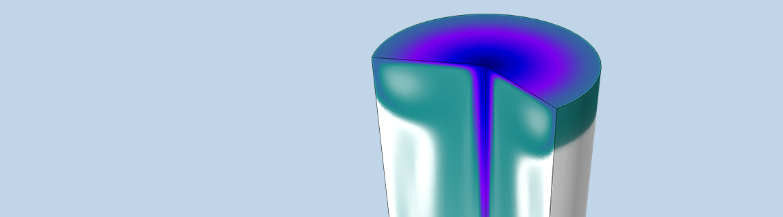
Comparing plots at t = 0 s and t = 10 s in the figure below, it is clear that the carbon dioxide bubbles, quantified by the gas volume fraction, start rising up in the water and impart momentum to the water. The carbon dioxide bubbles exit through the top surface. However, as water does not flow out through the top surface, it starts recirculating in the glass leading to the vortex formations observed in the figures below. The mass transfer takes place in the region where the gas volume fraction is nonzero, so initially, the aqueous carbon dioxide concentration closely follows the gas volume fraction. However, the aqueous carbon dioxide is carried by convection and diffusion to the remaining portion of the glass. The predominance of convective transport is evident when you compare the velocity, including streamlines, and the aqueous carbon dioxide concentration surface plots below.

Velocity magnitude of water along with the streamlines (left), carbon dioxide bubble volume fraction (center) and aqueous carbon dioxide concentration (right) at t = {0, 10, 50, 100} s.

In COMSOL Multiphysics, we can also create and export an animation of the plots above. This facilitates better visualization of the formation of vortices, their evolution in time, and the transport of the diluted species.

Time evolution of the velocity magnitude of water along with the streamlines (left), carbon dioxide bubble volume fraction (center), and aqueous carbon dioxide concentration (right).

As this is a 2D axisymmetric simulation, the COMSOL Multiphysics software automatically creates a 3D data set, which is a revolution of the 2D data set from the computed study. We can then create a 3D animation of the time evolution of carbonic acid, where the formation and transport of carbonic acid strongly follow the transport of aqueous carbon dioxide.

Time evolution of carbonic acid concentration.

Concluding Remarks

In this blog post, we discussed how to model sparging with an example of the carbonation of water. In general, a similar process can be used to model mass transfer between any two fluids in dispersed multiphase flows. Note that the Mass Transfer condition is available both in the Bubbly Flow and the Mixture Model interfaces. As is usually the case with COMSOL Multiphysics, you can also specify user-defined expressions under the Mass Transfer condition by scrolling down the list under Mass transfer model.

While modeling such multiphysics problems, it is useful to start with a simple model and then increase complexity for an optimal modeling workflow.

Next Steps

Interested in modeling sparging? Download a carbonation example by clicking the button below.

For more information on modeling dispersed and separated multiphase flows, check out these example models:

• Flow in an Airlift Loop Reactor
• Inkjet
• Free Surfaces with Level Set, Phase Field, and Moving Mesh: A Comparison

References

1. Sander, R., Compilation of Henry’s law constants for inorganic and organic species of potential importance in environmental chemistry, Air Chemistry Dept., Max-Planck Inst. of Chemistry, 1999.
2. Hogendoorn, J.A., Bhat, R.V., and Versteeg, G.F., “On the Determination of the Diffusivity of CO 2 in Aqueous and NonAqueous Solvents: Investigations with Laminar Jets and Wetted Wall Columns”, Chemical Engineering Communications, vol. 189, no. 8, pp. 1009–1037, 2002.
3. Han, J., Eimer, D.A., and Melaaen, M.C., “Liquid phase mass transfer coefficient of carbon dioxide absorption by water droplet”, Energy Procedia, vol. 37, pp. 1728–1735, 2013.