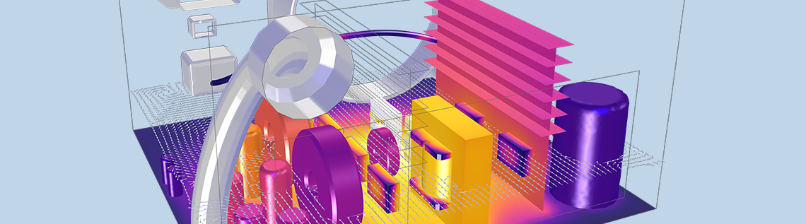
Whenever we have a heated or cooled part exposed to air, there is some transfer of heat from the part to the air via convection. The movement of the air can be either forced, via a fan, or free, as a result of the natural buoyancy variations due to changes in the air temperature. Today, we will look at several different ways of modeling these types of convection in the COMSOL Multiphysics® software.
Starting Simple: The Heat Transfer Coefficient
Let’s start by considering a model of the electrical heating of a busbar, shown below. You may recognize this as an introductory example to COMSOL Multiphysics, but if you haven’t already modeled it, we encourage you to review this model by going through the Introduction to COMSOL Multiphysics PDF booklet.
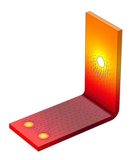
Electric currents (arrow plot) flowing through a metal busbar lead to resistive heating that raises the temperature (color surface plot).
In this example, we model electric current flowing through a busbar. This leads to resistive heating, which in turn causes the temperature of the busbar to rise. We assume that there is only heat transfer to the surrounding air, neglecting any conductive heat transfer through the bolts and radiative heat transfer. The example also initially assumes that there isn’t any fan forcing air over the busbar. Thus, the transfer of heat to the air is via natural, or free, convection.
As the part heats the surrounding air, the air gets hotter. As the air gets hotter, its density decreases, causing the hot air to rise relative to the cooler surrounding air. These free convective air currents increase the rate of heat transfer from the part to the surrounding air. The air currents depend on the temperature variations as well as the geometry of the part and its surroundings. Convection can, of course, also happen in any other gas or liquid, such as water or transformer oil, but we will center this discussion primarily around convection in air.
We can classify the surrounding airspace into one of two categories: Internal or External. Internal means that there is a finite-sized cavity (such as an electrical junction box) around the part within which the air is reasonably well contained, although it might have known air inlets and outlets to an external space. We then assume that the thermal boundary conditions on the outside of the cavity and at the inlets and outlets are known. On the other hand, External implies that the object is surrounded by what is essentially an infinitely large volume of air. We then assume that the air temperature far away from the object is a constant, known value.
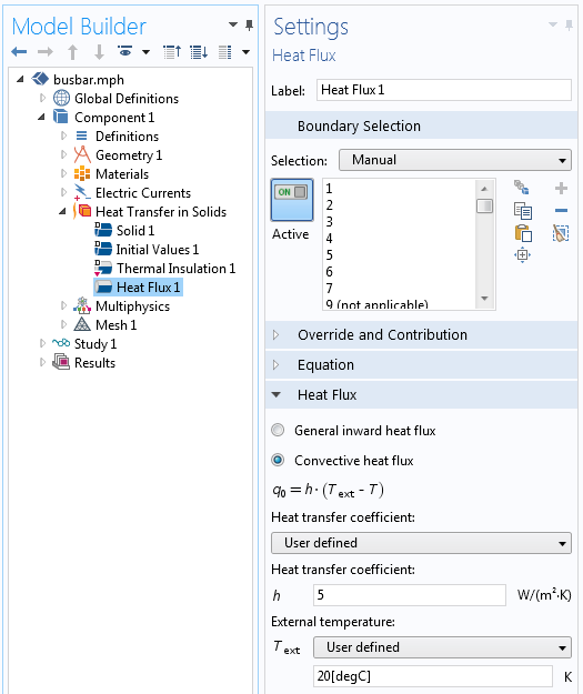
The settings for a constant heat transfer coefficient.
The introductory busbar example assumes free convective heat transfer to an external airspace. This is modeled using the following boundary condition for the heat flux:
where the external air temperature is Text = 25°C and h=5 W/m^2K is the heat transfer coefficient.
This single-valued heat transfer coefficient represents an approximate and average of all of the local variations in air currents. Even for this simple system, any value between h\approx 2-25 W/m^2K could be an appropriate heat transfer coefficient, and it’s worth trying out the bounding cases and comparing results.
If we instead know that there is a fan blowing air over this structure, then due to the faster air currents, we use a heat transfer coefficient of h\approx 10-250 W/m^2K to represent the enhanced heat transfer.
If the surrounding fluid is a liquid such as water, then the range of free and forced heat transfer coefficients are much wider. For free convection in a liquid, h\approx 50-1,000 W/m^2K is the typical range. For forced convection, the range is even wider: h\approx 50-20,000 W/m^2K.
Clearly, entering a single-valued heat transfer coefficient for free or forced convection is an oversimplification, so why do we do it? First, it is simple to implement and easy to compare the best and worst cases. Also, this boundary condition can be applied with the core COMSOL Multiphysics package. However, there are some more sophisticated approaches available within the Heat Transfer Module and CFD Module, so let’s look at those next.
Using a Convective Correlation
A convective correlation is an empirical relationship that has been developed for common geometries. When using the Heat Transfer Module or CFD Module, these correlations are available within the Heat Flux boundary condition, shown in the screenshot below.
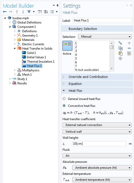
The Heat Flux boundary condition with the external natural convection correlation for a vertical wall.
Using these correlations requires that you enter the part’s characteristic dimensions. For example, with our busbar model, we use the External natural convection, Vertical wall correlation and choose a wall height of 10 cm to model the free convective heat flux off of the busbar’s vertical faces. We also need to specify the external air temperature and pressure. These values can be loaded from the ASHRAE database, a process we describe in a previous blog post.
The table below shows schematics for all of the available correlations. They take the information about the surface geometry and use a Nusselt number correlation to compute a heat transfer coefficient. For the horizontally aligned faces of the busbar, for example, we use the Horizontal plate, Upside and Horizontal plate, Downside correlations.
When using the Forced Convection correlations, you must also enter the air velocity. These convective correlations have the advantage of being a more accurate representation of reality, since they are based on well-established experimental data. These correlations lead to a nonlinear boundary condition, but this usually results in only slightly longer computation times than when using a constant heat transfer coefficient. The disadvantage is that they are only appropriate to use when there is an empirical relationship that is reasonable for the part geometry.
| Free Convection | Forced Convection | |
|---|---|---|
| External |  |
 |
| Internal |  |
 |
The available Convective Correlation boundary conditions.
Note that all of the above convective correlations, even those classified as Internal, assume the presence of an infinite external reservoir of fluid; e.g., the ambient airspace. The heat carried away from the surfaces goes into this ambient airspace without changing its temperature, and the ambient air coming in is at a known temperature. If, however, we are dealing with convection in a completely enclosed container, then none of these correlations are appropriate and we must move to a different modeling approach.
Approximating Free Convection in an Enclosure Using an Enhanced Thermal Conductivity
Let’s consider a rectangular air-filled cavity. If this cavity is heated on one of the vertical sides and cooled on the other, then there will be a regular circulation of the air. Similarly, there will be air circulation if the cavity is heated from below and cooled from above. These cases are shown in the images below, which were generated by solving for both the temperature distribution and the air flow.
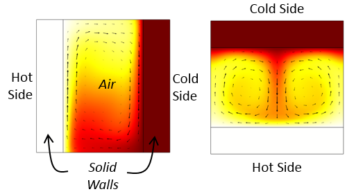
Free convective currents in vertically and horizontally aligned rectangular cavities.
Solving for the free convective currents is fairly involved. See, for example, this blog post on modeling natural convection. Therefore, we might like to find a simpler alternative. Within the Heat Transfer Module, there is the option to use the Equivalent conductivity for convection feature. When using this feature, the effective thermal conductivity of the air is increased based upon correlations for the horizontal and vertical rectangular cavity cases, as shown in the screenshot below.
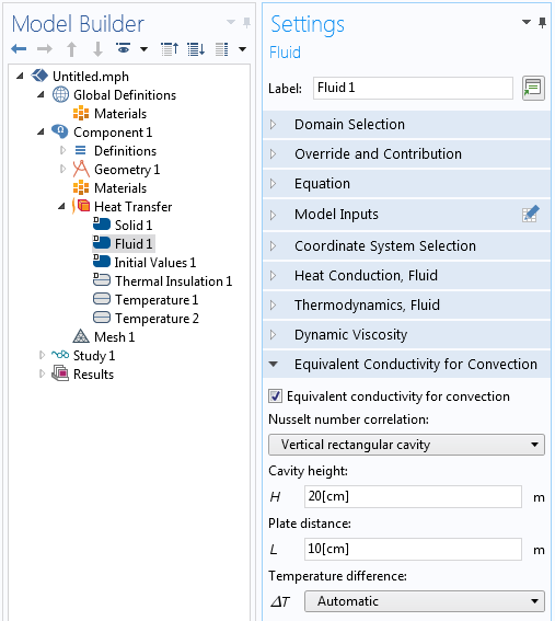
The Equivalent conductivity for convection feature and settings.
The air domain is still explicitly modeled using the Fluid domain feature within the Heat Transfer interface, but the air flow fields are not computed and the velocity term is simply neglected. The thermal conductivity is increased by an empirical correlation factor that depends on the cavity dimensions and the temperature variation across the cavity. The dimensions of the cavity must be entered, but the software can automatically determine and update the temperature difference across the cavity.
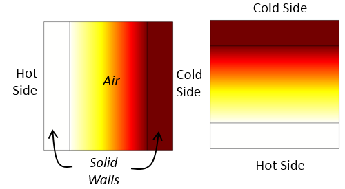
Temperature distribution in vertically and horizontally aligned cavities using the Equivalent conductivity for convection feature. The free convective air currents are not computed. Instead, the thermal conductivity of the air is increased.
This approach for approximating free convection in a completely closed cavity requires us to mesh the air domain and solve for the temperature field in the air, but this usually adds only a small computational cost. The disadvantage of this approach is that it is not very applicable for nonrectangular geometries.
Approximating Forced Convection in an Enclosure Using Isothermal Domains
Next, let’s consider a completely sealed enclosure, but with a fan or blower inside that actively mixes the air. We can reasonably assume that well-mixed air is at a constant temperature throughout the cavity. In this case, it is appropriate to use the Isothermal Domain feature, which is available with the Heat Transfer Module when the Isothermal domain option is selected in the Settings window.

The settings associated with using the Isothermal Domain interface.
A well-mixed air domain can be explicitly modeled using the Isothermal Domain feature. In the model, the temperature of the entire domain is a constant value. The temperature of the air is computed based upon the balance of heat entering and leaving the domain via the boundaries. The Isothermal Domain boundaries can be set as one of the following options:
- Thermally Insulated: no heat transfer across the boundary
- Continuity: continuity of temperature across the boundary
- Ventilation: a known mass flow of fluid, of known temperature, into or out of the isothermal domain
- Convective Heat Flux: a user-specified heat transfer coefficient, as described earlier
- Thermal Contact: a specific thermal resistance
Of all of these boundary condition options, the Convective Heat Flux is the most appropriate for well-mixed air in an enclosed cavity.
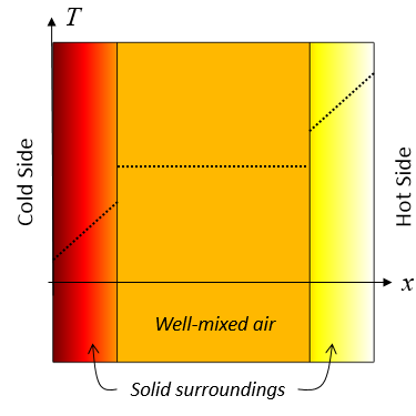
Representative results when using an Isothermal Domain feature. The well-mixed air domain is a constant temperature and there is heat transfer to the surrounding solid domains via a specified heat transfer coefficient.
Modeling the Airflow Explicitly
The most computationally expensive approach, but also the most general, is to explicitly model the airflow. We can model both forced and free convection as well as simulate an internal or external flow. This type of modeling can be done with either the Heat Transfer Module or CFD Module.
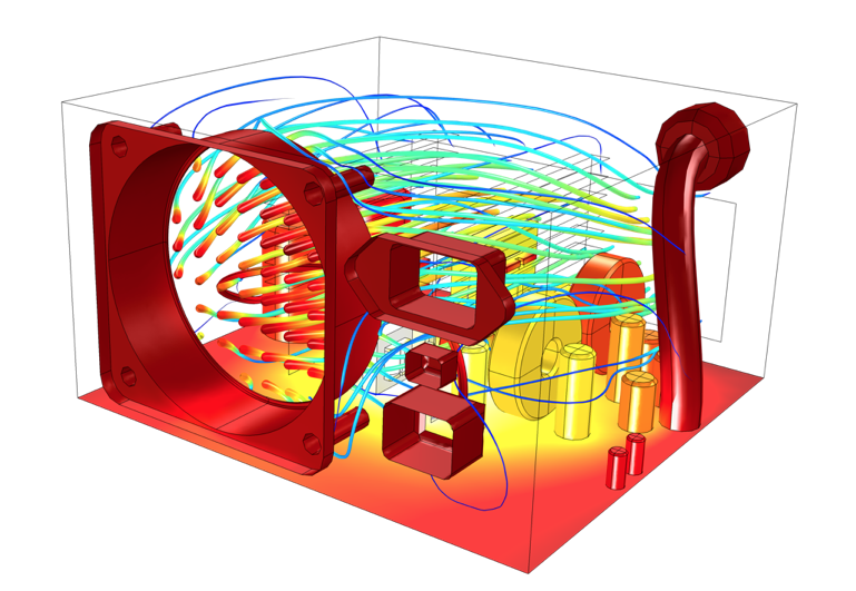
An example of computing air flow and temperature within an enclosure.
If you finished the Introduction to COMSOL Multiphysics booklet, you have already solved one example of an internal forced convection model. You can learn more about explicitly modeling airflow in the resources mentioned at the end of this post.
When Can We Ignore Free Convection Entirely?
We will finish up this topic by addressing the question: When can free convection in air be ignored and how can we model these cases? When a cavity’s dimensions are very small, such as a thin gap between parts or a very thin tube, we run into the possibility that the viscous damping will exceed any buoyancy forces. This balance of viscous to buoyancy forces is characterized by the nondimensional Rayleigh number. The onset of free convection can be quite varied depending on boundary conditions and geometry. A good rule of thumb is that for dimensions less than 1mm, there will likely not be any free convection, but once the dimensions of the cavity get larger than 1cm, there likely will be free convective currents.
So how can we model heat transfer through these small gaps? If there is no air flow, then these air-filled regions can simply be modeled as either a solid or a fluid with no convective term. This is demonstrated in the Window and Glazing Thermal Performances tutorial. It is also appropriate to model the air as a solid within any microscale enclosed structure.
If these thin gaps are very small compared to the other dimensions of the system being analyzed, you can further simplify the gaps by modeling them via the Thin Layer boundary condition with a Thermally thick approximation layer type. This boundary condition introduces a jump in temperature across interior boundaries based on the specified thickness and thermal conductivity.
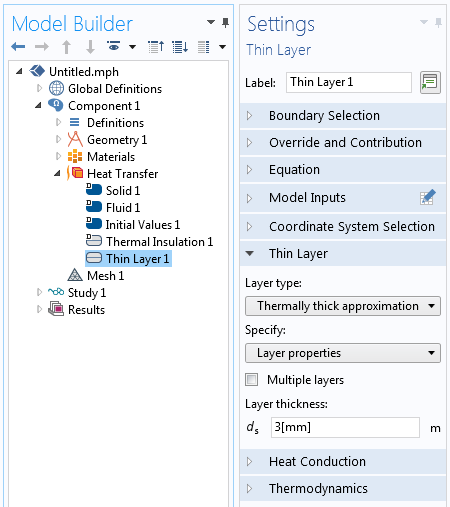
The Thin Layer boundary condition can model a thin air gap between parts.
We can use the previous two approaches within the core COMSOL Multiphysics package. In the Heat Transfer Module, there are additional options for the Thin Layer condition to consider more general and multilayer boundaries, which can be composed of several layers of materials.
Closing Remarks on Modeling Natural and Forced Convection in COMSOL Multiphysics®
Before closing out this discussion, we should also quickly address the question of radiative heat transfer. Although we haven’t discussed radiation here, an engineer must always take it into consideration. Surfaces exposed to ambient conditions will radiate heat to the surroundings and be heated by the Sun. The magnitude of radiative heating from the Sun is significant — about 1000 watts per square meter — and should not be neglected. For details on modeling radiative heat transfer to ambient conditions, read this previous blog post.
There will also be radiative heat transfer between interior surfaces. Radiative heat flux between surfaces is a function of the difference of temperature to the fourth power. Keep in mind that radiative heat transfer between two surfaces at 20°C and 50°C will be 200 watts per square meter at most, but rises to 1000 watts per square meter for surfaces at 20°C and 125°C. To correctly compute the radiative heat transfer between surfaces, it is also important to compute the view factors with the Heat Transfer Module.
Today we looked at several approaches for modeling convection, starting from the simplest approach of using a constant convective heat transfer coefficient. We then discussed using an Empirical Convective Correlation boundary condition before going over how to use an effective thermal conductivity within a domain and an isothermal domain feature, approaches with higher accuracy and only a slightly greater computational cost. The most computationally intensive approach — explicitly computing the flow field — is, of course, the most general. We also touched on when it is appropriate to neglect free convection entirely and how to model such situations. You should now have a greater understanding of the available options and trade-offs for modeling free and forced convection. Happy modeling!
Additional Resources
- Learn about explicitly modeling air flow and heat transfer on the COMSOL Blog
- Get an introduction to simulating heat transfer in an archived webinar


Comments (7)
Moustafa AlDamook
November 23, 2017Incredible blog
many thanks for this effort
Jonathan Meza
July 19, 2018About the constant heat transfer coefficient… “the external air temperature is Text = 25°C h=5 W/m2K” have you the references of the constants or the convection heat transfer coefficient in a lab
Moustafa AlDamook
September 17, 2018Dear Walter,
Could you help me, I am stuck in modelling the air free convection in enclosure. If this possible could i send to you my model to check where is the error please?
Best regards
Moustafa
Rahul Karmankar
May 14, 2025Dear sir,
I have some queries regarding the direction of flow in forced convection. I have a 3D object using the Z-axis type for geometry construction.
When I want to apply heat flux for any boundary in forced convection, it asks for length and velocity. I want to maintain same flow of velocity throughout
the object, regardless of boundaries, means I want to use the fan from any one of the corners of the object, which shows the same direction of flow.Pleasee suggest me how can I obtain it ?
Walter Frei
May 14, 2025 COMSOL EmployeeRegarding the above question, these would be best addressed within the scope of COMSOL Technical Support. Please reach out via: https://www.comsol.com/support
Piotr Markowski
November 27, 2025And what about modelling using air (fluid) velocity as an input data instead of directly written heat transfer coefficient? Is it possible for COMSOL to calculate heat transfer coefficient?
Walter Frei
December 1, 2025 COMSOL EmployeeHello Piotr,
Yes, the External Forced, and Internal Forced Convection Correlation boundary conditions give the correlations for a Plate, Cylinder, Sphere, and Pipe flow (respectively) heat transfer coefficients, where the user can enter the fluid velocity.
Happy Modeling!