Rotordynamics Module

Analyze the Dynamics of Rotating Machinery

When designing machinery with rotating parts, it is of great importance that the effects of spinning are captured correctly. Accurate simulations help engineers better determine how to avoid system breakdown and failure, as well as how to best optimize operation and performance. The Rotordynamics Module, an add-on to the Structural Mechanics Module, is specifically designed for performing simulations of rotating machinery, providing the capabilities needed for such decision-making.

The study of rotordynamics is important in application areas that involve rotating machinery. These include, for example, the automotive and aerospace industries, power generation, and the design of electrical products and household appliances. With the multiphysics capabilities of the COMSOL® software, modeling can be used to simulate fatigue, analyze sound propagation, and investigate the interactions between stationary and moving components, such as the interactions between a spinning shaft and hydrodynamic bearings.

Contact COMSOL
A gas turbine model in the Prism color table.

Analyze Rotor–Bearing Systems

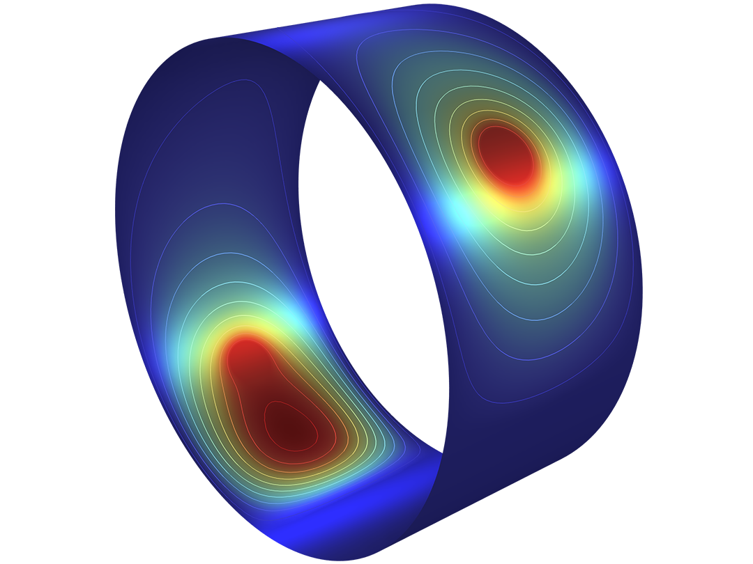
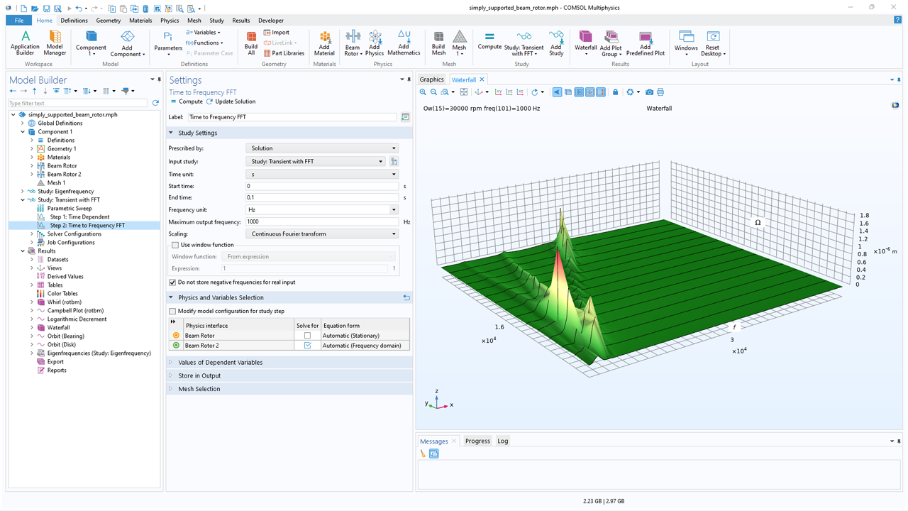
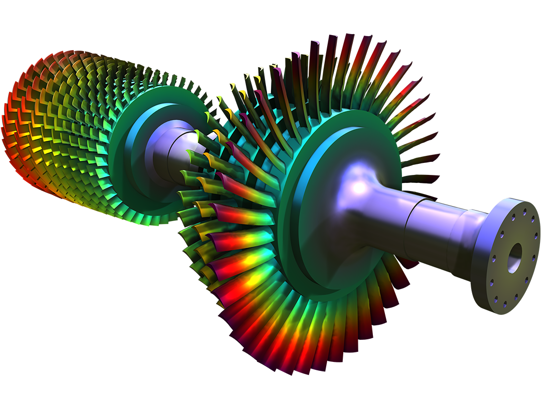
The physical behavior of rotating machines is greatly influenced by vibrations, which are exacerbated by the spinning and shape of the machines themselves. Even perfectly symmetrical rotor assemblies exhibit mode separation with increasing rotational speed. This implies that the usual behavior of identical modes in perpendicular symmetry planes is not applicable for rotating shafts. In addition, even minor imperfections and imbalances can give rise to significant vibration amplitudes when operating close to the natural frequencies of the rotating system.

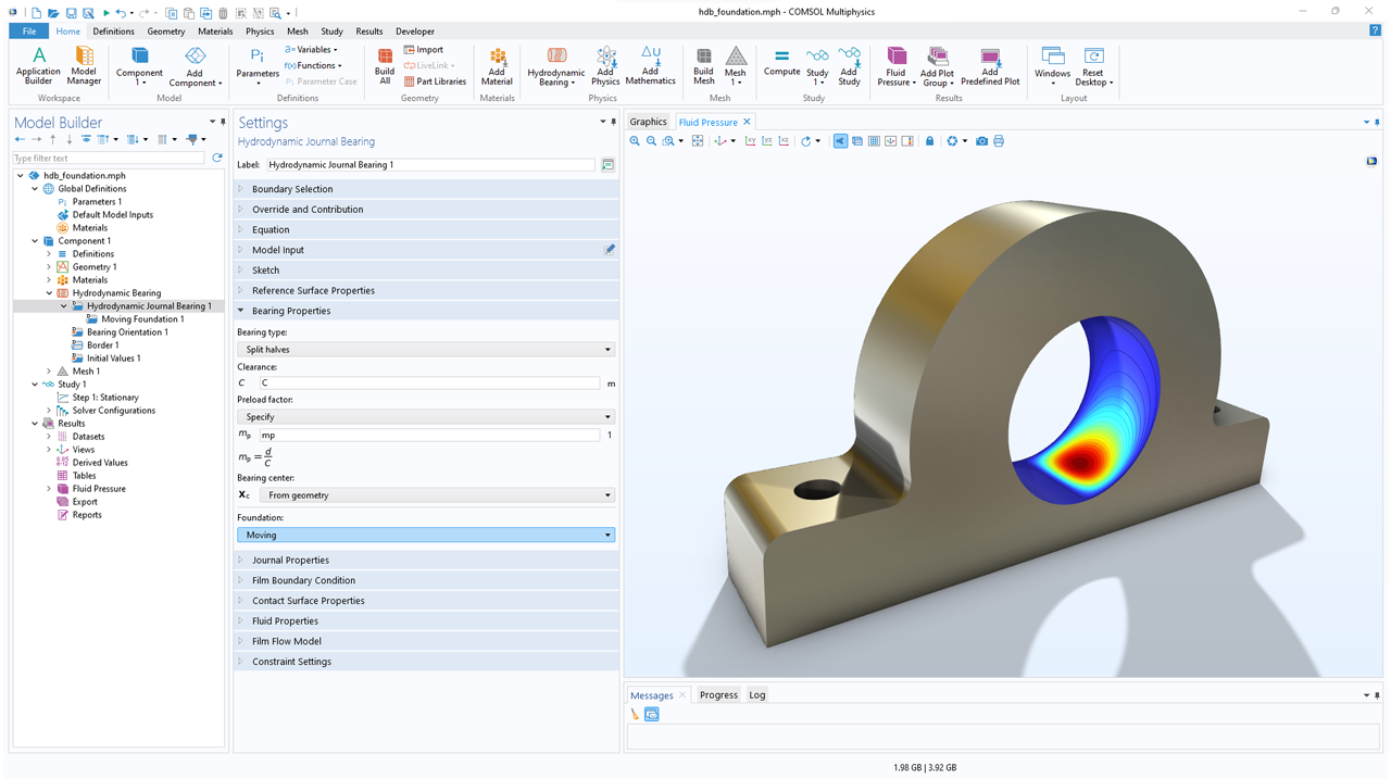
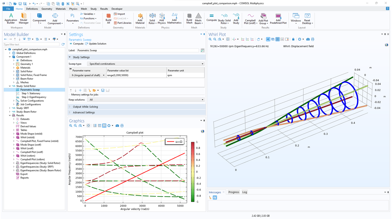
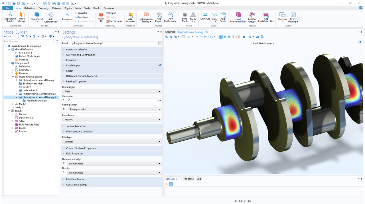
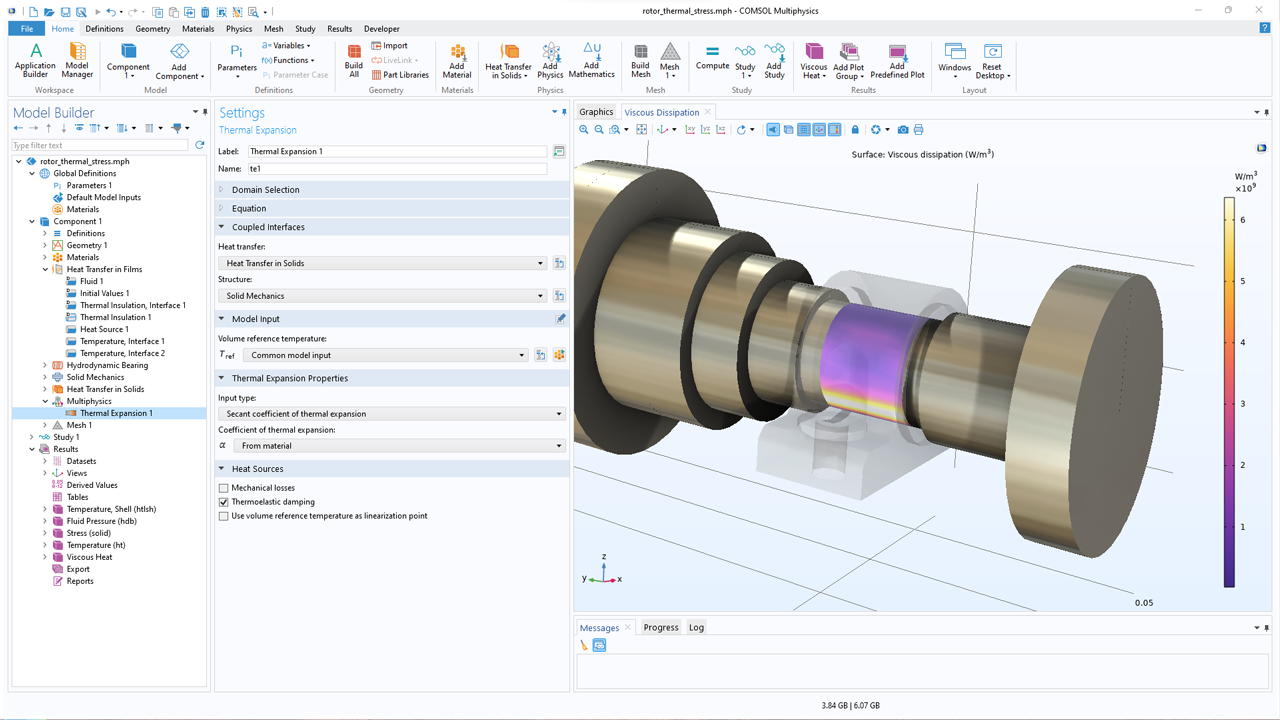
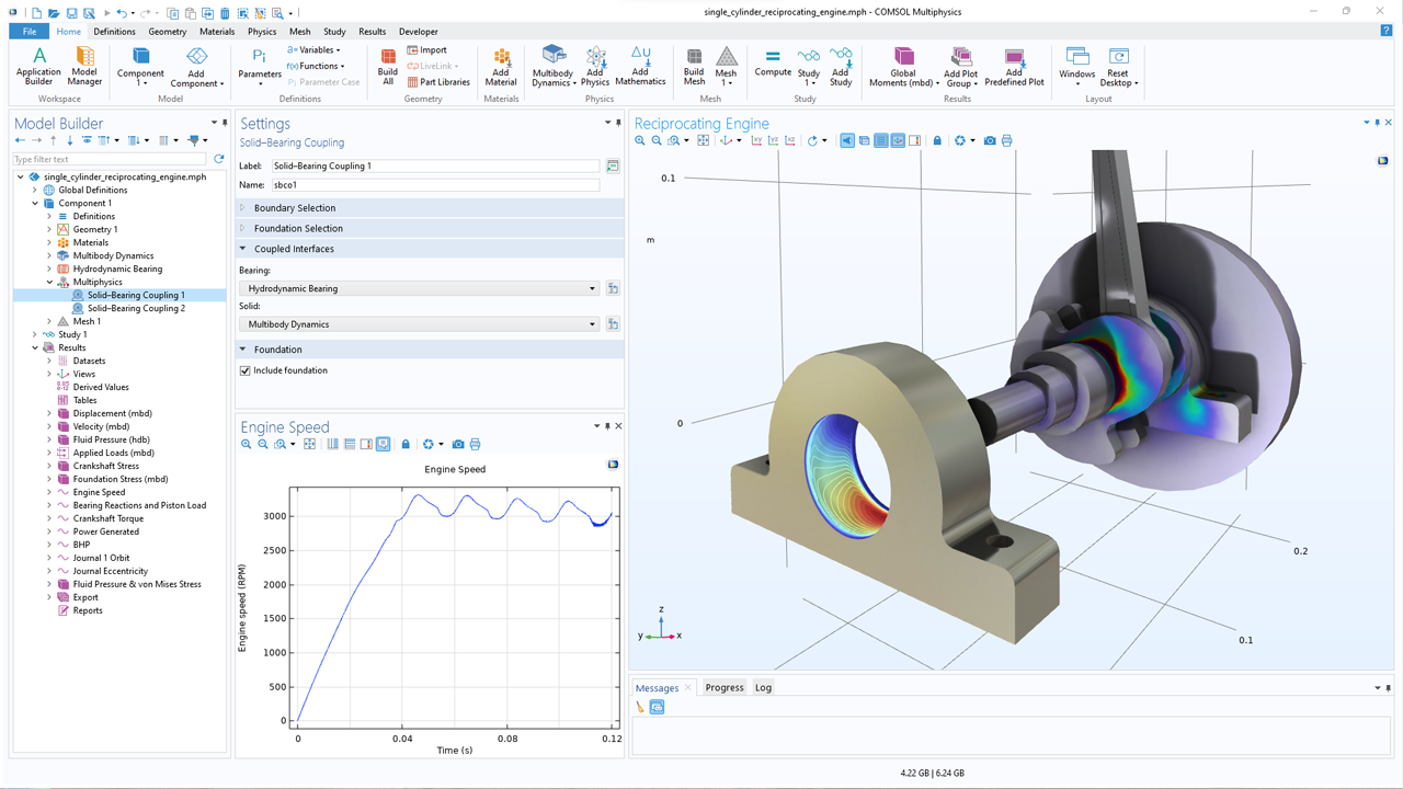
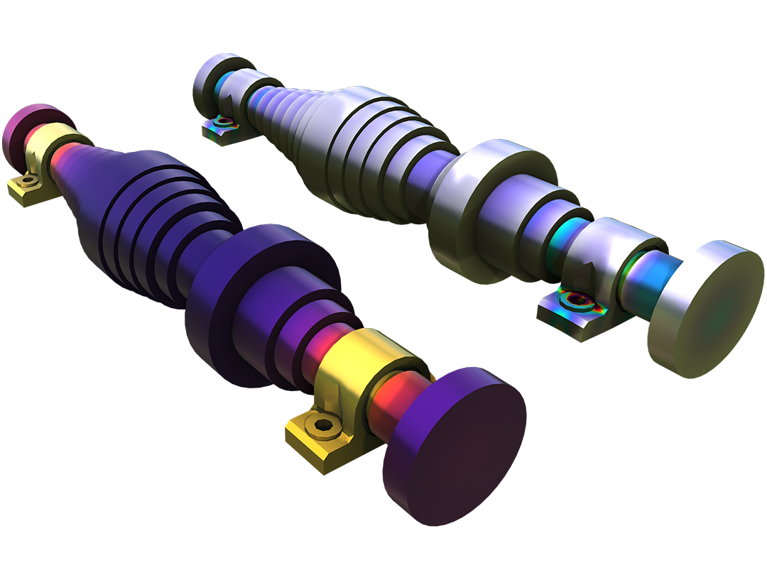
The Rotordynamics Module enables the analysis of resonances, stresses, and strains in rotors, bearings, disks, and foundations, allowing users to keep conditions within acceptable operating limits. The module can also be used to evaluate how different design parameters influence natural frequencies and, consequently, the critical speeds, whirl, and stability thresholds. Moreover, it can be used to investigate the stationary and transient unbalance responses.

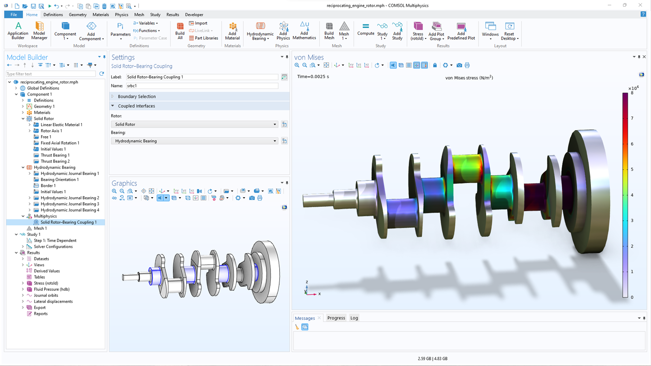
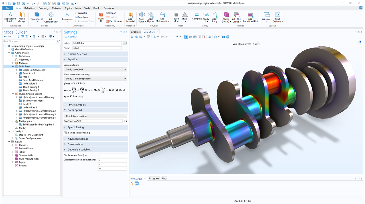
The module also provides capabilities that can be used to predict how the rotational behavior may lead to stresses in the rotor itself and to transmissions of loads and vibration to other parts of the rotating machine's assembly.

Hydrodynamic Bearing Simulations

In order for a rotating machine to cross critical speeds, it is important to have sufficient damping. For this reason, hydrodynamic bearings are often used to support the spinning shafts. In the Rotordynamics Module, the behavior of hydrodynamic bearings can be analyzed in detail.

Depending on the compliance and geometry of the bearing surfaces, the bearing loading, and the lubricant properties, different effects must be taken into account to determine the supporting pressure distribution. With the Rotordynamics Module, simple hydrodynamic simulations can be performed, or the module can be combined with the Structural Mechanics Module and Heat Transfer Module to perform more complex elastohydrodynamic or thermo-elastohydrodynamic simulations.

Features and Functionality in the Rotordynamics Module

Perform various rotordynamic simulations in the COMSOL Multiphysics® software.

A close-up view of the Model Builder with the Solid Rotor node highlighted and a turbocharger model in the Graphics window.

Built-In User Interfaces

The COMSOL Multiphysics® simulation platform and its add-on modules offer a set of predefined interfaces for specific physics areas. The Rotordynamics Module provides dedicated interfaces for accurately modeling rotors and bearings. The Solid Rotor interface is used for modeling a rotor as a full 3D geometric model made with CAD software or using the built-in CAD capabilities of COMSOL Multiphysics®. The Beam Rotor interface offers a less computationally expensive method, where the rotor can be modeled as a 1D beam and the rotor components can be implemented as points within the model.

The Solid Rotor and Beam Rotor interfaces can be used to compute displacements, velocities, accelerations, and stresses. For detailed modeling of a bearing that includes lubricant film, a Hydrodynamic Bearing interface is available.

A close-up view of the Model Builder with the Beam Rotor node highlighted and a motor drive model in the Graphics window.

Beam Rotors

Modeling rotor systems quickly becomes computationally expensive. Therefore, it is common practice to simplify the representation of the shaft. In many cases, the overall dynamics of a rotor can be sufficiently modeled by using a specialized beam element.

For this type of analysis, a line representation is applied, which uses an effective geometrical description governed by the shaft's cross-section properties. This approach can be particularly useful, for example, when dealing with rotor systems consisting of axisymmetric shafts with ideally rigid disks. The beam rotor model can also be used for simulations of rotor rub in cases where rotor displacements are restricted.

A close-up view of the Settings window for the Radial Roller Bearing node and a gearbox model in the Graphics window.

Abstract Bearings

Often, rotors are supported by bearings to prevent lateral and/or axial movements at certain locations. In the Rotordynamics Module, a range of abstract bearings is provided, modeled using an implicit bearing description. This includes various types of bearings, such as:

  • Journal bearing
  • Thrust bearing
  • Radial roller bearing
  • Active magnetic bearing
  • Multi-spool bearing

Within these categories, multiple variations are available. Take, for example, the Radial Roller Bearing option, which may have single- and two-row variations, encompassing different bearing styles, such as:

  • Deep groove ball
  • Angular contact ball
  • Self-aligning ball
  • Spherical roller
  • Cylindrical roller
  • Tapered roller
A close-up view of the Hydrodynamic Journal Bearing settings and a foundation model in the Graphics window.

Foundations

The structural components on which rotor–bearing systems rest, sometimes referred to as the foundation, can be modeled at different levels of complexity. The foundation can be selected as:

  • Fixed
  • Flexible
  • Moving

When the foundation is significantly stiffer than the rotor and its supports, the Fixed Foundation option can be used, assuming that the bearing is rigidly fixed in space. Alternatively, the Flexible Foundation option imitates the flexibility of the foundation using a set of flexible springs. For scenarios where the movements of the bearing foundation need to be explicitly included, the Moving Foundation option can be selected.

A close-up view of the Model Builder with a Reduced Component node highlighted and a gearbox model in the Graphics window.

Component Mode Synthesis (CMS)

In the Rotordynamics Module, the Craig–Bampton method makes it possible to reduce linear components to computationally efficient reduced-order models. These components can then be integrated into a model consisting solely of reduced components or combined with nonreduced elastic finite element (FE) models, which can include nonlinear components. This technique, known as component mode synthesis or dynamic substructuring, significantly reduces both computation time and memory usage.

A close-up view of the Settings window for the Parametric Sweep node and a whirl plot in the Graphics window.

Results and Visualization

The Rotordynamics Module provides capabilities for creating clear and concise visualizations of simulation results and making the data available for future use and analysis. It also includes a variety of plot types that are specific to rotordynamics applications, including:

  • Whirl plots, which plot the mode shapes of a rotor rotating about the rotor axis at discrete rotation intervals
  • Campbell plots, which plot variations of the natural frequencies of the rotor with respect to rotor speed
  • Waterfall diagrams, which display variations of the frequency spectrum as functions of rotational speed
  • Orbit plots, which show displacement at certain rotor components (or points), such as at disks and bearings
A close-up view of the Solid Rotor–Bearing Coupling settings and a reciprocating engine model in the Graphics window.

Multiphysics Interfaces and Couplings

In the Rotordynamics Module, there are multiphysics couplings available that can be used capture the effects of oil whirl and whip. To model a 3D rotor with a hydrodynamic bearing and the interactions between them, the Solid Rotor with Hydrodynamic Bearing multiphysics interface can be used. This interface combines the Solid Rotor and Hydrodynamic Bearing interfaces through a Solid Rotor–Bearing Coupling multiphysics coupling. This coupling transfers the velocity and displacement information from the Solid Rotor interface to the Hydrodynamic Bearing interface.

To model a rotor defined as a beam and a hydrodynamic bearing, as well as the interactions between them, the Beam Rotor with Hydrodynamic Bearing multiphysics interface combines the Beam Rotor and Hydrodynamic Bearing interfaces through a Beam Rotor–Bearing Coupling multiphysics coupling.

A close-up view of the Model Builder with the Solid Rotor node highlighted and a reciprocating engine model in the Graphics window.

Solid Rotors

In some applications, it is not possible to ignore factors such as rotor asymmetries, cross-sectional deflections, or the dynamics of disks, blades, and other attachments. In these cases, the geometry can be explicitly modeled using a full 3D representation of the rotor.

This approach automatically captures the effects of spin softening and stress stiffening through its underlying continuum description, offering the most accurate depiction of how rotors behave under various conditions.

A close-up view of the Model Builder with a Hydrodynamic Journal Bearing node highlighted and a crankshaft model in the Graphics window.

Hydrodynamic Bearings

For more advanced simulations of rotors supported by fluid film bearings, the Hydrodynamic Bearing interface can be used. This interface enables the investigation of the pressure distribution, velocity field, and power losses in a fluid film. When using liquids as lubricant, simple analyses with the Reynolds equation can be performed or cavitation can be taken into account with the Jakobsson–Floberg–Olsson (JFO) cavitation theory. For gas-lubricated bearings, a modified Reynolds equation is used.

The interface can be used for modeling various predefined types of bearings and dampers, or even types specified by the user. The predefined types include:

  • Hydrodynamic journal bearing:
    • Plain
    • Elliptical
    • Split halves
    • Multilobe
    • Tilting pad
  • Hydrodynamic thrust bearing:
    • Step
    • Tapered land
    • Tilting pad
  • Floating ring bearing
  • Squeeze film damper

It is also possible to specify inlets, outlets, or bearing misalignments to represent the bearing at hand.

A close-up view of the Thermal Expansion settings and a rotor model in the Graphics window.

Material Models

In the Rotordynamics Module, the Linear Elastic Material feature is used as a default material model. This feature adds equations for the displacements in a linear elastic rotor and can define the elastic and inertial properties of a material. The equations in this feature account for the frame acceleration forces induced by the rotation of the rotor. Many other effects can be incorporated as well, such as thermal expansion, initial and external stresses and strains, and damping.

A close-up view of the Model Builder with the Time to Frequency FFT node highlighted and a waterfall plot in the Graphics window.

Study Types

The Rotordynamics Module offers a variety of study types for both static and dynamic analyses of rotor assemblies. This includes parametric studies for exploring a rotor's behavior under different conditions, such as varying mass eccentricities, using a Stationary study. The Eigenfrequency study, alternatively, is particularly useful for identifying stable operating ranges and critical speeds by conducting repeated eigenfrequency analyses across a range of rotational speeds.

For scenarios where all loads on the rotor are time harmonic, the Frequency Domain study computes the rotor's response. A Time Domain study can be used when considering the inertial effects of imbalances and their temporal changes relative to the corotating frame.

A Transient with FFT study performs a parametric sweep over a rotor's angular speed and includes a time-domain simulation followed by a fast Fourier transform (FFT). This study type is computationally expensive but is advantageous when subsynchronous and supersynchronous vibrations in the rotor–bearing system are predominant.

A close-up view of the Model Builder with the Solid−Bearing Coupling node highlighted and a reciprocating engine model in the Graphics window.

Extended Multiphysics Analyses

The Rotordynamics Module can be combined with other products in the COMSOL product suite to perform coupled simulations and multiphysics analyses. This enables in-depth examination of various physical effects on a rotor system. For instance, by combining the Rotordynamics Module with the Multibody Dynamics Module, transient simulations can be conducted to predict vibrations in a geared rotor assembly when it's subjected to external torque. Similarly, for assessing the fatigue life of stator and rotor components, the Rotordynamics Module can be seamlessly combined with the Fatigue Module.

Every business and every simulation need is different.

In order to fully evaluate whether or not the COMSOL Multiphysics® software will meet your requirements, you need to contact us. By talking to one of our sales representatives, you will get personalized recommendations and fully documented examples to help you get the most out of your evaluation and guide you to choose the best license option to suit your needs.

Just click on the "Contact COMSOL" button, fill in your contact details and any specific comments or questions, and submit. You will receive a response from a sales representative within one business day.

Next Step

Request a Software Demonstration