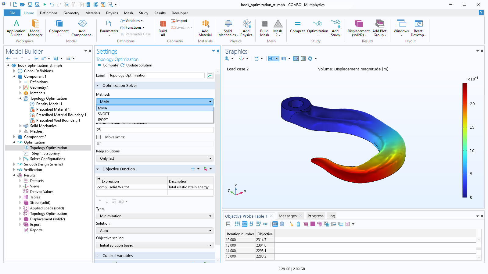
Structural Topology Optimization
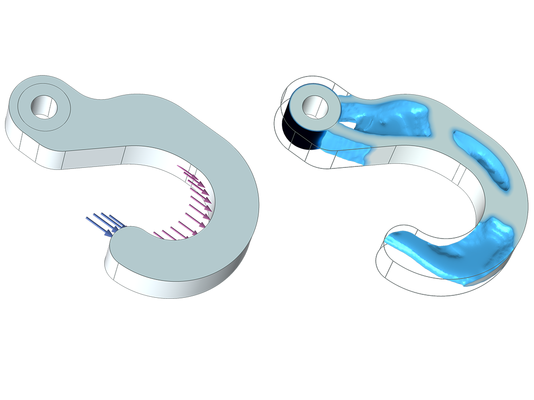
Topology optimization of a hook, where the material is distributed for optimal compliance for a given total weight.
Optimize Multiphysics Models
The Optimization Module, an add-on to COMSOL Multiphysics®, provides tools for parameter, shape, and topology optimization, as well as parameter estimation. It can be used together with other modules from the COMSOL product suite to optimize devices and processes that involve phenomena such as electromagnetics, structural mechanics, acoustics, fluid flow, heat transfer, and more. Geometric dimensions can be optimized when the Optimization Module is combined with the CAD Import Module, Design Module, or any of the LiveLink™ products for CAD.
Starting with an objective function to improve and a set of design variables to change, along with an optional set of constraints, the software will search for an optimal design. Any inputs to the model — whether geometric dimensions, part shapes, material properties, or material distribution — can be treated as design variables, and any model output can be used as the objective function, which is then minimized or maximized.
Contact COMSOL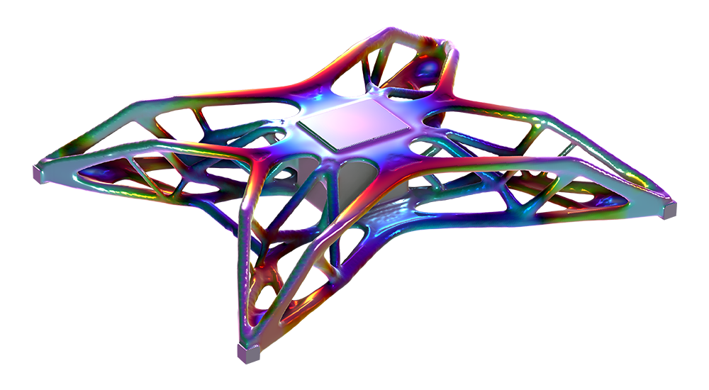
The Optimization Module can be combined with any of the COMSOL® add-on products for optimization in different areas of physics.
Topology optimization of a hook, where the material is distributed for optimal compliance for a given total weight.
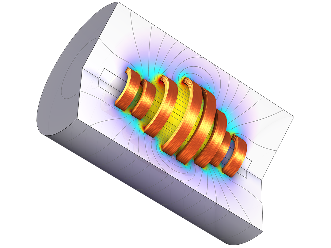
Parameter and shape optimization of a ten-turn coil, optimized with respect to the magnetic flux density and power dissipation.
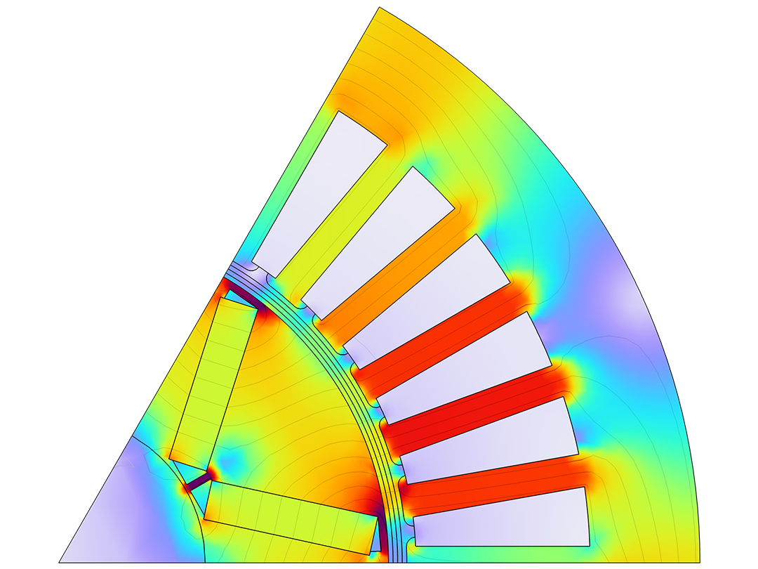
Parameter optimization of an electric motor to identify the best position and shape of the permanent magnets based on torque.

Topology optimization of a magnetic circuit used in a loudspeaker driver for reduced large-displacement nonlinear response.

Shape optimization of a loudspeaker tweeter dome and waveguide achieves a flatter response curve and improved radiation pattern.
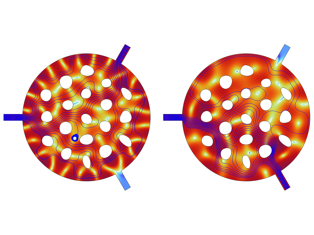
Shape optimization of an acoustic demultiplexer: The acoustic energy goes to different output ports for different frequency bands.
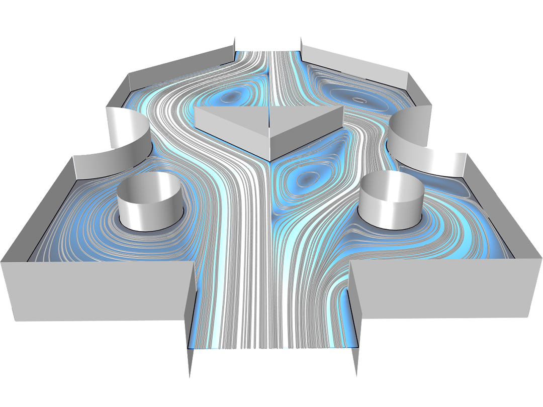
Parameter, shape, and topology optimization for a Tesla microvalve maximizing the ratio of the pressure drop for the bidirectional flow.
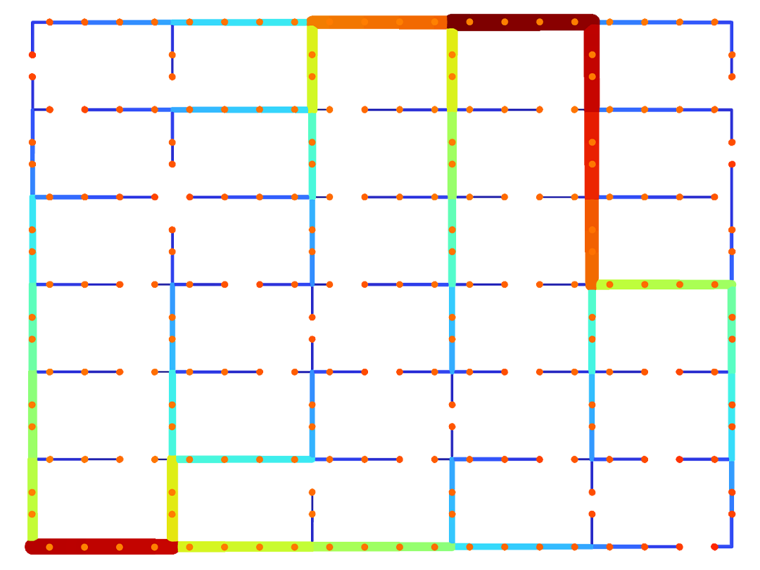
Topology optimization of a district heating network layout.
COMSOL Multiphysics® provides specialized user interfaces with dedicated solvers for the available types of optimization.
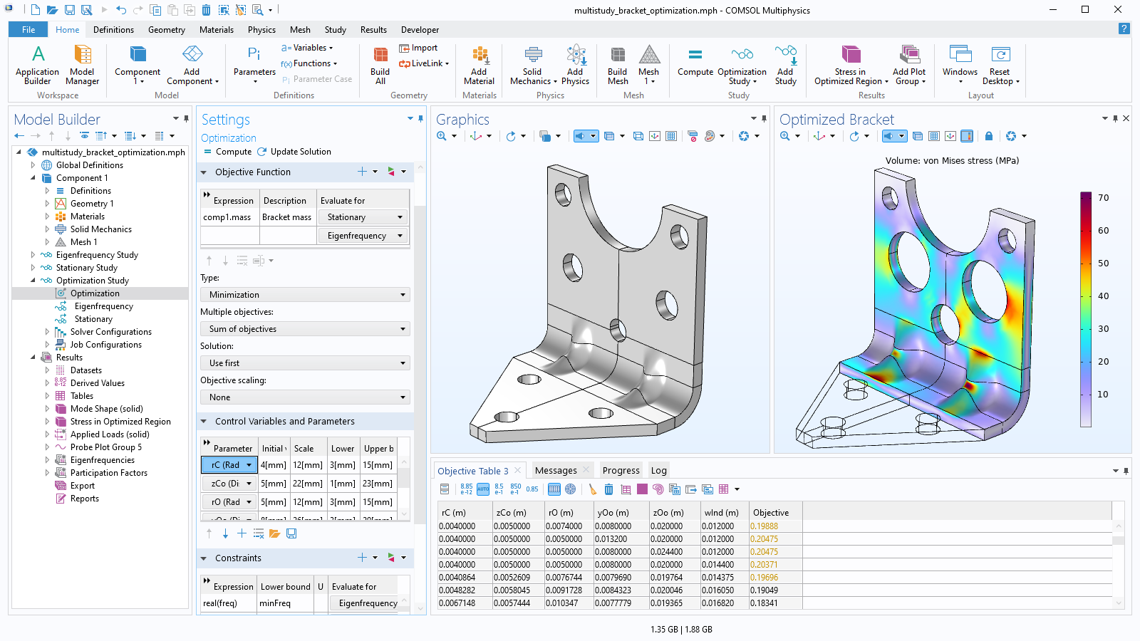
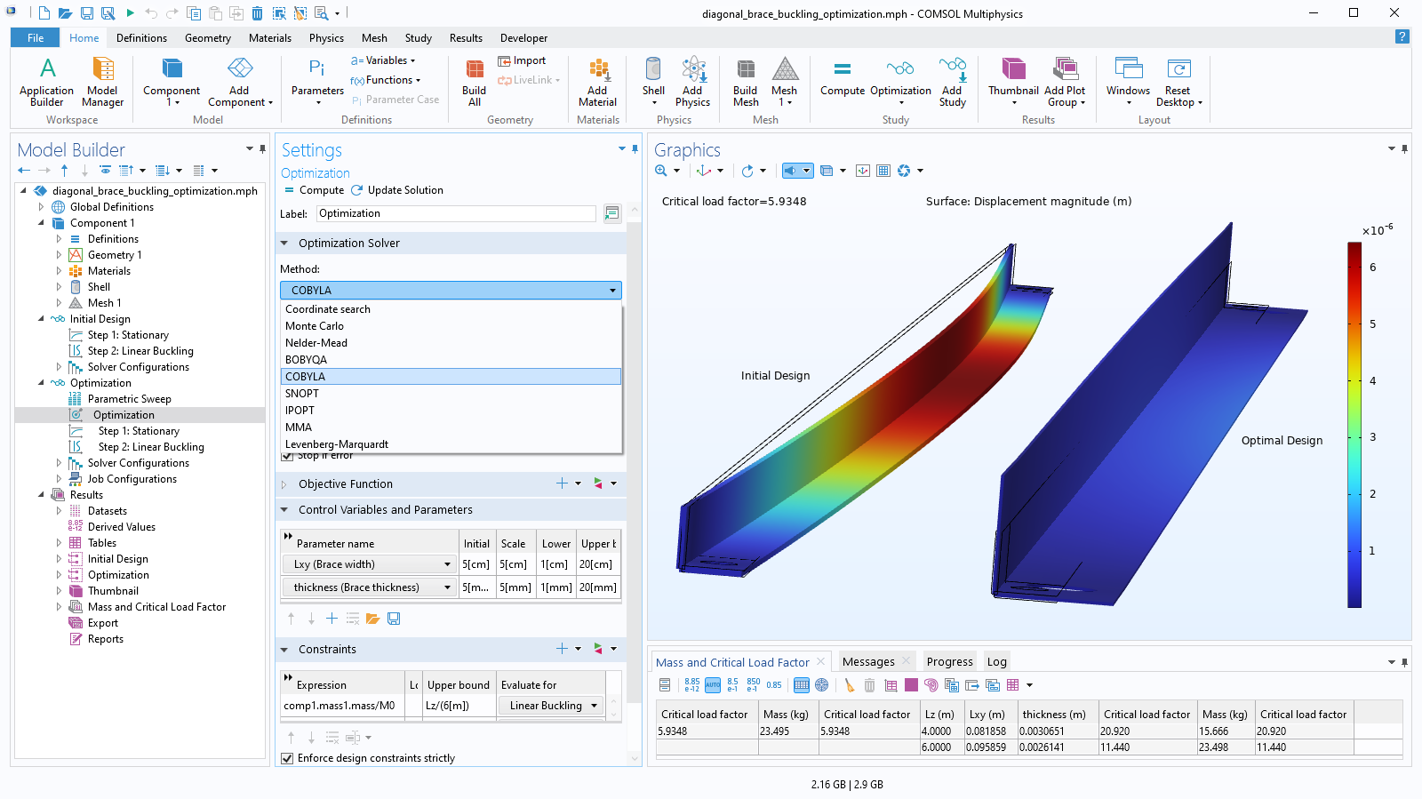
To set up a parameter optimization in COMSOL Multiphysics®, only a general-purpose Optimization study needs to be added. An associated settings window prompts the user to add an objective function, control variables and parameters, and constraints. The parameters used for parameter optimization can be the same that were used to set up the model in the first place, such as geometry dimensions, material properties, or boundary loads. Whereas a parametric sweep will provide an overview of the design parameter space, a parameter optimization will provide the optimal parameters and objective function values.
When running a parameter optimization with parameters that define geometry dimensions, remeshing is needed at each iteration — a process that is fully automatic with the Optimization Module. The optimal solution is always a true CAD part that can be immediately exported to industry-standard CAD formats. This functionality requires the CAD Import Module, the Design Module, or one of the LiveLink™ products for CAD.

Topology optimization represents even greater freedom in geometry variation than both parameter and shape optimization. This approach allows for the removal and addition of material during the optimization process, allowing holes to be created in the geometry that were not originally present in the design. This method typically results in an organic-looking design, making it a popular method for light weighting. A dedicated user interface and study are available for topology optimization.
The extreme design freedom associated with topology optimization may result in designs that cannot be manufactured with conventional methods. It is therefore common to introduce manufacturing constraints, as this enables the optimized design to be produced using, for example, extrusion or milling.
Like with shape optimization, remeshing is not required for topology optimization. The optimal and smoothed design is made available in the STL, 3MF, or PLY file formats for further use in another software program or for verification analysis within COMSOL Multiphysics®.
Gradient-based optimization methods are used when the derivatives can be computed efficiently using the adjoint method. This is possible for custom objectives or constraints, as long as these are differentiable. Symbolic differentiation in the COMSOL Multiphysics® software's core technology makes this possible, providing the flexibility needed for custom multiphysics analyses.
Gradient-based optimization can be used when a design problem has thousands, or even millions, of variables. This is often the case for shape or topology optimizations, where the design variables represent field quantities that are distributed throughout space and represented by different values in each mesh element.
The gradient-based methods simultaneously compute all analytic derivatives, whereas the derivative-free methods have to approximate each derivative and therefore take more time as the number of design variables increases.
The gradient-based methods included in the Optimization Module are:
They are supported for the following types of studies:
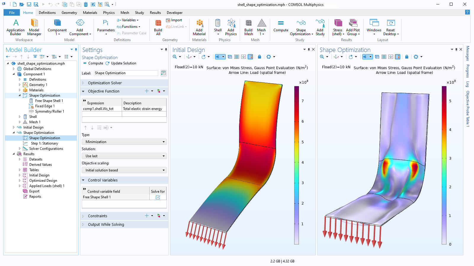
As an alternative to varying a set of CAD parameters, the built-in features for shape optimization can be used to allow the geometry to deform either more or less freely. This approach allows for greater freedom and can sometimes produce even better results than parameter optimization. A set of dedicated user interfaces is available for easily defining the allowed deformations of boundaries in a 2D or 3D model. Additionally, a specialized shell shape optimization feature is available, as well as a shape optimization study type for controlling the solvers.
The tools used for shape optimization in solids are based on methods that deform the mesh in a controlled manner, where remeshing is not required. The optimal geometry is available in a faceted surface mesh format, such as STL, 3MF, or PLY. This geometry can then be reused in a separate analysis in COMSOL Multiphysics® or exported for use in another software.

A model is only as accurate as its input, but it can be difficult to source accurate material parameters from suppliers. To account for nonlinearities, experiments may need to be performed. However, it can be challenging to design experiments from which the desired parameters can be extracted using analytical methods.
A solution to these problems is to use the parameter estimation functionality of the Optimization Module to find the set of parameters of a model that minimizes the deviation between the physical and the simulated experiment. In addition to the interface for general parameter estimation, a specialized user interface for curve fitting is available for fitting a curve (represented by a model expression) to time-dependent data.
The parameter estimation method is based on least-squares fitting and can be used when the reference data is a function of time or a single parameter. In many cases, an estimate of the variance and confidence of the estimated parameters will be provided.
To get started with parameter estimation, a ready-to-use app is available. Users can import measurement data or use the app's built-in tutorial samples, as well as enter custom model expressions to fit the curve.
Derivative-free optimization methods are used when the search directions needed by the optimization solver can only be computed indirectly. This is often the case for parameter optimization, where the control variables represent geometry dimensions and remeshing is needed at each iteration step.
The derivative-free methods included in the Optimization Module are:
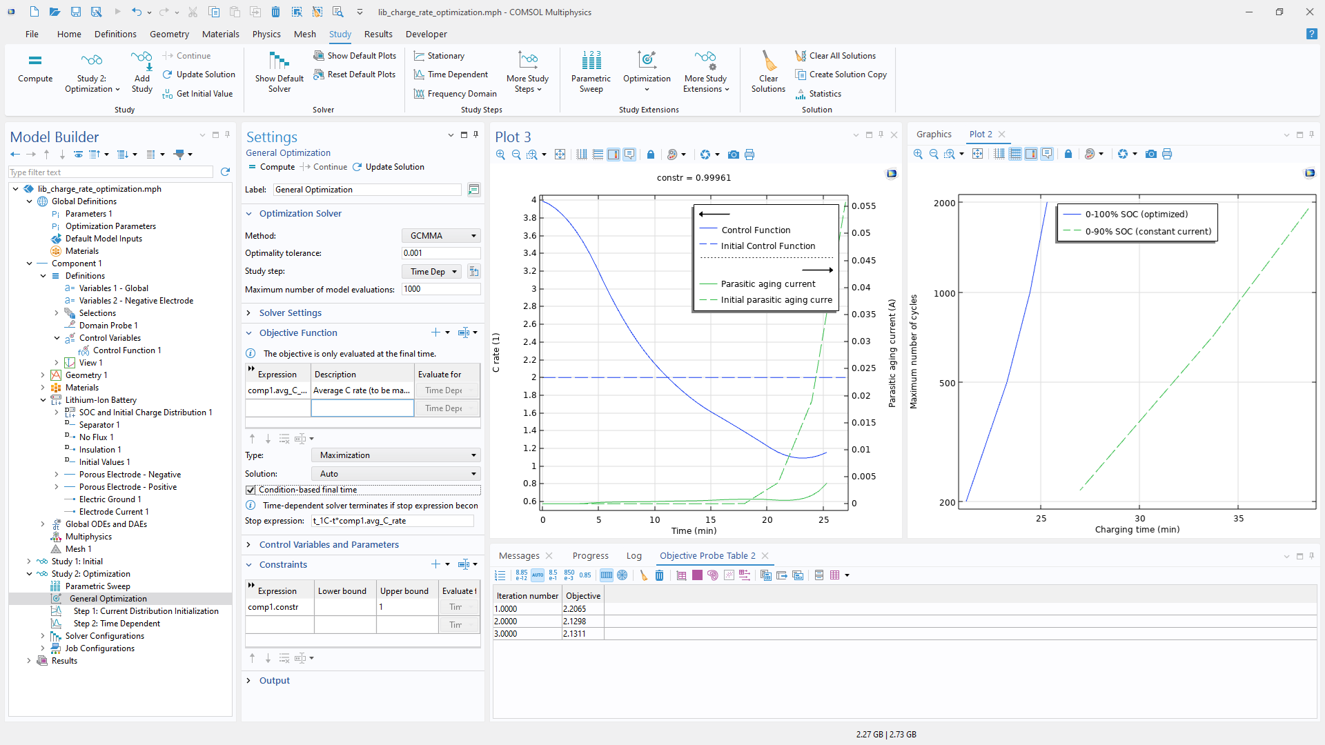
Process duration is often tied to cost, so minimizing time can lead to cost reductions. In other cases, however, it can be beneficial to maximize the duration of process, for example, the degradation or breakdown of a product.
The Optimization Module includes built-in support for common optimal control formulations, which includes regularization and convenient export of the optimized control values. This functionality makes it easy to set up a problem, solve it, and reuse the results in a larger simulation or workflow.
Both optimal control and time-optimal control are supported with all optimization solvers. However, substantial improvements often require many adjustable parameters, which is best addressed using gradient-based optimization methods.
Using the Application Builder together with the Optimization Module opens the door for a wider set of users to run optimization studies independently, without the need to consult a simulation expert.
For example, optimization models can include parameter estimation based on experimental data; an app tailored to this particular task would enable a user to input various sets of experimental data without worrying about the details of the optimization model itself.
Using apps also offers a more efficient workflow for optimal control. The Optimization Module can be used to identify which transient input generates a desired transient output. In such cases, users may want to adjust the desired output based on experimental results. Creating an app for this task packages the complexity of this process into a custom user interface, allowing various users to run optimal control simulations simply by specifying their desired outputs.
Every business and every simulation need is different.
In order to fully evaluate whether or not the COMSOL Multiphysics® software will meet your requirements, you need to contact us. By talking to one of our sales representatives, you will get personalized recommendations and fully documented examples to help you get the most out of your evaluation and guide you to choose the best license option to suit your needs.
Just click on the "Contact COMSOL" button, fill in your contact details and any specific comments or questions, and submit. You will receive a response from a sales representative within one business day.
Request a Software Demonstration