
When analyzing optical designs, it is essential to consider not only light intensity but also polarization. Careful manipulation of light polarization can greatly improve image quality by filtering out light from unwanted sources — for example, to minimize glare. A useful way to learn about light polarization, and how to manipulate it, is through a Fresnel rhomb. With the COMSOL Multiphysics® software, engineers can model the effect of a Fresnel rhomb and similar elements on light polarization in optical systems.
Manipulating Linearly and Circularly Polarized Light
In the early 1800s, Augustin-Jean Fresnel, known for his research and inventions in the field of optics, was the first scientist to describe light as linearly, circularly, or elliptically polarized. In a linearly polarized plane electromagnetic wave, the two transverse components of the electric field are in phase with each other. We can think of these components as sine or cosine functions that reach their maximum at the same position and also reach zero at the same position. The following plot shows a linearly polarized wave; the electric field of the wave itself is shown in yellow, whereas the x– and y-components are shown in red and green, respectively.
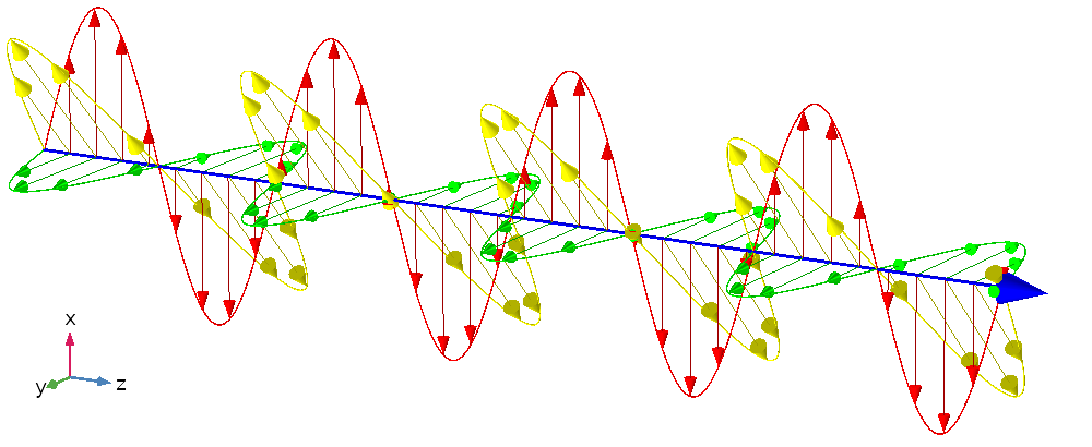
A linearly polarized plane electromagnetic wave.
Compare this linearly polarized wave to the circularly polarized wave shown below. Here, the x– and y-components of the electric field are equal in magnitude but are offset by a 90° phase delay. Thus, when one component reaches a maximum or minimum value, the other is zero. The net effect is that the sum of these two components has a spiral-like shape, hence the name “circular polarization”.
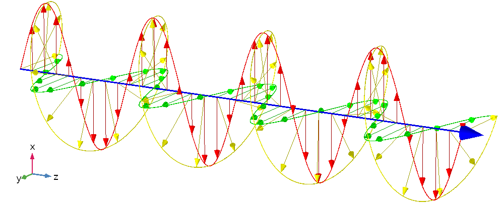
A circularly polarized plane electromagnetic wave. The x– and y-components are shown in red and green, respectively. The direction of propagation is in blue, and the total electric field amplitude is in yellow.
Fresnel’s discovery of linearly and circularly polarized radiation lent support to his hypothesis that light is a pure transverse wave (with no longitudinal component), meaning that the oscillations of the electric and magnetic fields are always perpendicular to the direction of propagation. By further studying light polarization, he was able to explain that the total internal reflection (TIR) of light does not depolarize incident linearly polarized light, as previously thought, but rather changes it to elliptically or circularly polarized light. The production of circularly polarized light by TIR can be conveniently demonstrated by a glass parallelepiped in which light undergoes TIR at two opposite faces — a setup now known as a Fresnel rhomb.
A Fresnel rhomb is a type of glass prism that manipulates the polarization of light. The incident light is linearly polarized at a 45° angle to the plane of incidence. The light then undergoes TIR at two different faces. Each instance of TIR causes a phase delay of 45° between the electric field components polarized in the plane of incidence and perpendicular to it, for a total phase delay of 90°. Thus, the outgoing light is circularly polarized.
By using COMSOL Multiphysics® and the add-on Ray Optics Module, engineers can predict the polarization of light as it propagates through an optical system. This is because the Ray Optics Module records light intensity and polarization using the Stokes–Mueller calculus, or simply Mueller calculus, which can fully represent any state of polarization. In the next section, let’s look at a tutorial model that demonstrates light changing from linearly to circularly polarized at a specific angle of incidence in a Fresnel rhomb.
Modeling a Fresnel Rhomb with COMSOL Multiphysics®
The Fresnel rhomb geometry is a simple uncoated glass prism in the shape of a parallelepiped. A simple diagram of the geometry is given below.
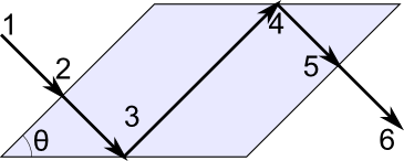
Linearly polarized light (1) enters the prism (2). This light is linearly polarized 45° to the plane of incidence — that is, the components of the electric field lying in the screen and perpendicular to it have equal magnitudes, and they are in phase. The prism has an angle (θ) that, if set properly, will cause a 45° phase delay between the orthogonal electric field components during each instance of TIR (3 and 4). The light then exits the prism (5). The outgoing light (6) is now circularly polarized. The components of the electric field lying in your screen and perpendicular to it still have equal magnitudes, but they are now 90° out of phase.
The exact value of the phase delay caused by TIR on an uncoated surface depends on the refractive indices on either side of the surface, n1 and n2, and on the angle of incidence, θ. The relationship between these quantities and the phase delay can be derived from Snell’s law and the Fresnel equations. (For more details about the equations, you can check the Fresnel Rhomb model documentation.)
2 \times \textrm{atan}\left(\frac{\cos\theta\sqrt{\sin^2\theta – \left(n_2/n_1\right)^2}}{\sin\theta}\right) = 45^{\circ}
The model consists of two studies. First, the value of θ that gives the desired phase delay of 45° is solved for. Then, this angle is used to define the geometry for the ray optics simulation.
Study 1: Solving for the Angle of Incidence
First, you can use the Global ODEs and DAEs interface to solve the above equation for the angle of incidence that causes a phase retardation of δ = 45° between the s– and p-polarized components during each TIR for the refractive index ratio of n = 1/1.51. (Even though this equation is not an ordinary differential equation or differential-algebraic equation, you can still use this interface to solve it.) The resulting value of θ in this example is 0.84855 radians or ~48.618°.
Study 2: Tracing the Path of the Light Ray
Next, you can use the Geometrical Optics interface to trace the path of a light ray through the Fresnel rhomb as it undergoes TIR at the angle of incidence computed by the Global ODEs and DAEs interface. Note that the ray is linearly polarized at this stage, with its direction of polarization at a 45° angle to the plane of incidence.
The value for the angle of incidence obtained from Study 1 (0.84855 radians) can be used to set up the model geometry for the Fresnel rhomb, which is a parallelogram extruded into a 3D geometry. Using a 3D geometry is preferred because it helps to illustrate the state of ray polarization, since the 3D Ray Trajectories plot can display polarization ellipses. In this step, the Stokes parameters, which are computed along each ray trajectory, are used to describe the degree to which a ray is linearly or circularly polarized.
Evaluating the Simulation Results
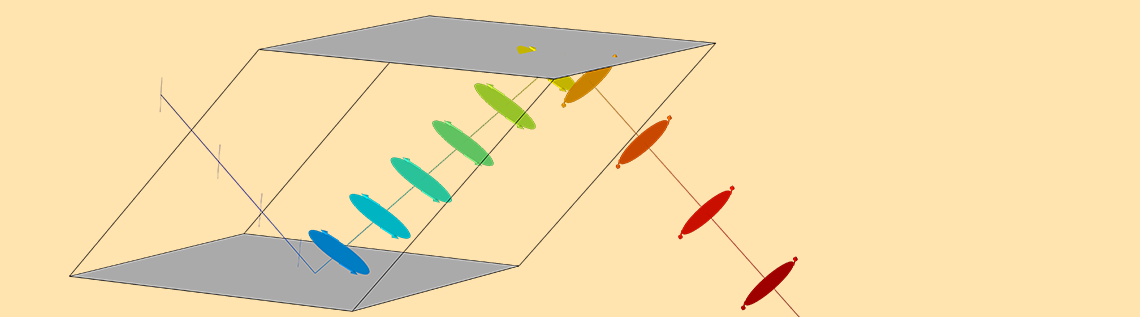
Now, let’s take a closer look at the simulation results in the aforementioned Ray Trajectories plot. In this plot, shown below, the linear ray enters from the left side of the prism. The colors illustrate the optical path length along the ray, and the circles and ellipses along the ray path show the polarization. The arrows along the perimeter of each circle/ellipse show the sense of rotation of the instantaneous field vector.
As the light goes through the Fresnel rhomb, the linearly polarized ray becomes elliptically polarized after one TIR. After two TIRs, the polarization ellipses change to circles, meaning the light is circularly polarized.
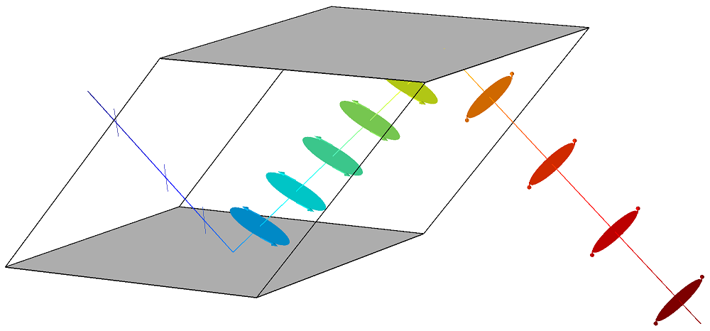
Ray propagation in a Fresnel rhomb.
At this camera angle, it might not be obvious that the outgoing light is circular. But by rotating the 3D plot in the Graphics window, you can see that the light changes from linear to elliptical to circular polarization.
Animation showing the incident light in a Fresnel rhomb when it is linearly polarized (δ = 0), elliptically polarized after one reflection (δ = 45°), and circularly polarized after two reflections, (δ = 90°).
You can visualize this polarization in another way by plotting the ratio of the Stokes parameters, the results of which are displayed below. To start, the ray is linearly polarized, with the ratio at zero. After the first TIR, the ratio has values with magnitudes between zero and one, indicating varying degrees of elliptical polarization. Then, after the second TIR, the magnitude is almost exactly unity, becoming more aligned with circular polarization.
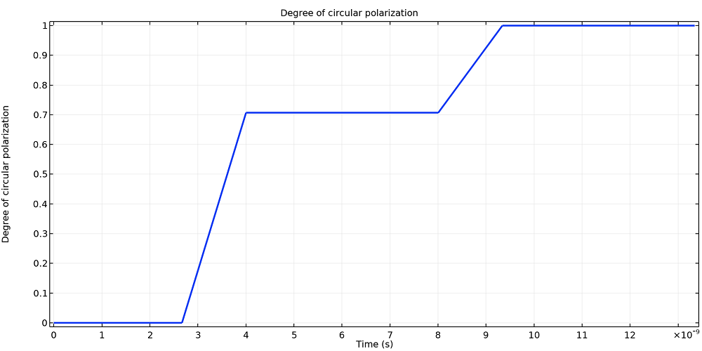
The ratio of the fourth and first Stokes parameters plotted as a function of the optical path length.
Next Steps
To try the Fresnel rhomb model featured in this blog post, click the button below. Then, in the Application Gallery, you can download the step-by-step documentation for this example and the accompanying MPH file.
A natural extension of the Fresnel rhomb tutorial is to apply thin dielectric coatings to the prism surfaces. Dielectric coatings affect the Fresnel coefficients at an interface; therefore, they can affect the phase delay between in-plane and out-of-plane electric field components. An example of this is a TIR thin-film achromatic phase shifter (TIRTF-APS). It uses thin films to offset the frequency dependence of the refractive index in the glass so that outgoing light remains circularly polarized for a wide range of wavelengths.
Further Reading
Want to learn more about ray optics modeling? Take a look at these blog posts:


Comments (0)