
In today’s blog post, we will introduce a procedure for thermally modeling a material with hysteresis, which means that the melting temperature is different from the solidification temperature. Such behavior can be modeled by introducing a temperature-dependent specific heat function that is different if the material has been heated or cooled past a certain point. We can implement this behavior in COMSOL Multiphysics via the Previous Solution operator and a little bit of equation-based modeling. Let’s find out how…
What Is Thermal Hysteresis and How Is It Modeled?
A material with thermal hysteresis will exhibit a solidification temperature that is different from the melting temperature. Such materials have applications in heat sinks and thermal storage systems and are even used by living organisms, such as fish and insects living in cold climates. We won’t concern ourselves here with the exact physical mechanisms by which thermal hysteresis happens, but rather focus on how to model it.
We will begin by considering a representative material with hysteresis that is incompressible and plot out the enthalpy of the material as a function of temperature, as shown below. When the material is in the solid state and is being heated, the enthalpy is given by the bottom curve or path. As the material passes the melting temperature, it becomes completely liquid. When this material is subsequently cooled in the liquid state, it will follow the upper path, thus the material remains liquid at temperatures below the melting temperature. Once the freezing temperature is reached, the material becomes completely solid. If the material is then heated back up, it will follow the bottom path, and so on. In the completely molten or completely solid state, the two enthalpy curves overlap. The latent heat of melting and solidification is the jump in these curves.
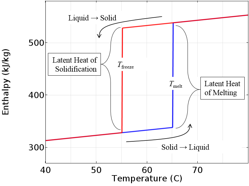
Enthalpy versus temperature for an idealized incompressible material.
Now, the above curve represents a bit of an idealized case that would only occur in the real world if we had a perfectly pure material. It is also a bit impractical for computational modeling purposes since this immediate transition between states represents a discontinuity that is quite difficult to solve numerically.
However, if we introduce a small transition zone over which the enthalpy varies smoothly, then we have a model that is much more amenable to numerical analysis. The physical interpretation of this is that the material changes phase over some finite temperature and in the intermediate range, the material is a mixture of both solid and liquid. Only once the material is fully outside of the transition zone will it switch over to following the other curve.
Note that we have centered the smoothing around the nominal melting and freezing temperatures, so the fully molten state is at a temperature slightly higher than the nominal melting temperature and the fully solid state is slightly below the freezing temperature. The plot below shows a gradual smoothing, but this transitional zone can be made very narrow to better approximate the behavior if we really did have a perfectly pure material.
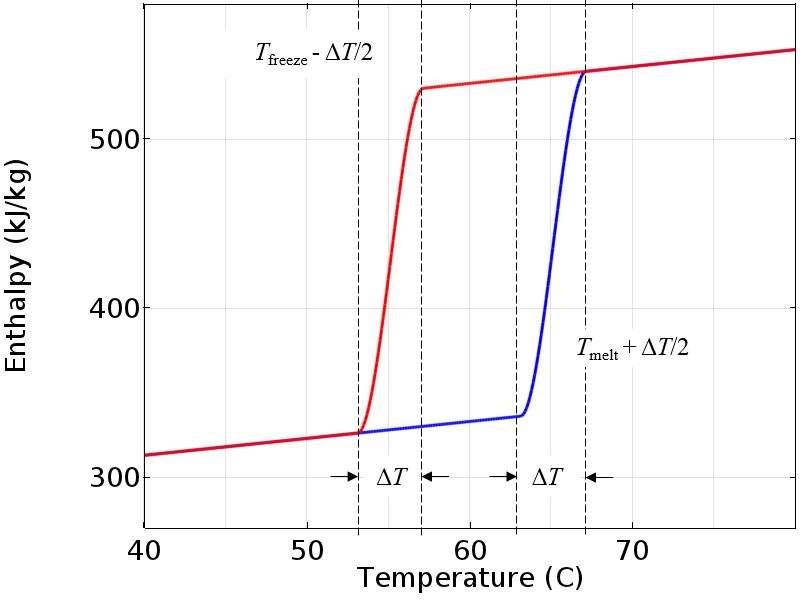
A smoothed enthalpy curve is more amenable to numerical analysis.
Since the material is assumed to be incompressible, the enthalpy depends only on the temperature. The above plot will also give us the specific heat, which is the derivative of enthalpy with respect to temperature. The specific heat is constant except for a small region around the melting and freezing temperatures.
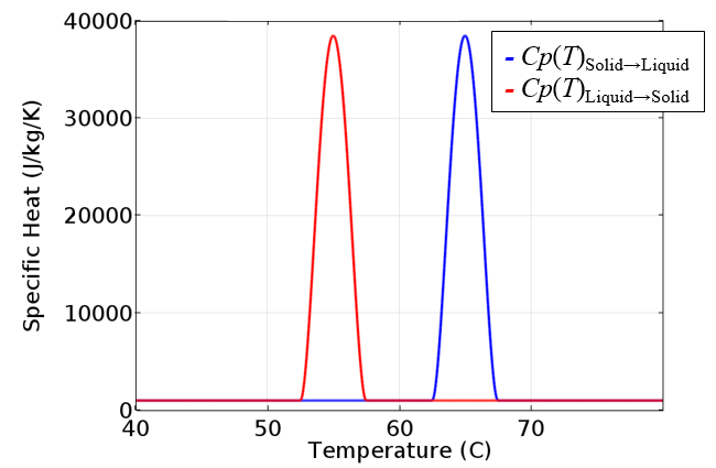
The specific heat is the derivative of the enthalpy with respect to temperature and is different if the material is heated or cooled.
This temperature-dependent specific heat data can be put directly into the governing equation for heat transfer and, along with an appropriate set of boundary conditions, can be solved in COMSOL Multiphysics. In fact, the existing Application Gallery example, Cooling and Solidification of Metal, makes use of such a temperature-dependent specific heat, albeit without hysteresis. The only additional requirement for modeling thermal hysteresis is to introduce a switch to determine which path to follow. Let’s now look at how to implement this in COMSOL Multiphysics.
Implementing Thermal Hysteresis in COMSOL Multiphysics
Here, we will look at a simple example model of a phase-change material within a thin-walled container. One side wall is perfectly insulated and the wall on the other side is held at a known temperature that varies periodically over time. A schematic of this is shown below. We are interested in computing the temperature as a function of time and position through the thickness and can reduce this to a one-dimensional model to get started.
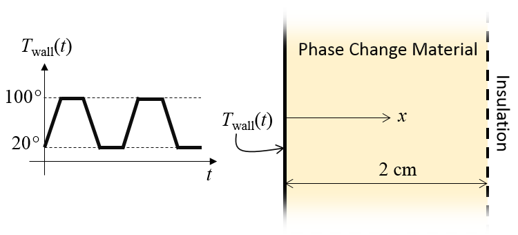
Schematic of the thermal model. A time-varying temperature is applied at one side.
Our modeling begins by setting up some physical constants via the Global Parameters that define the melting and freezing temperatures and the smoothing to apply to the enthalpy functions. The two smoothed enthalpy functions plotted earlier are implemented as shown in the screenshot below. We can here take advantage of the built-in Step function, which additionally features the option to apply a user-defined smoothing.
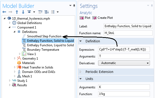
Implementation of the enthalpy functions shown above, using the smoothed step function. Note that the units have been defined.
The geometry of our model is simply a 1D interval representing the phase-change material region. The Heat Transfer in Solids interface is used, since we are assuming that there is no fluid flow. The material properties are as shown below.
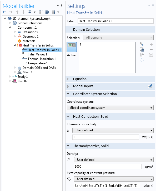
Screenshot showing the material properties definitions in the phase-change material.
The thermal conductivity and the density are constants. The specific heat (the heat capacity at constant pressure) is defined as:
SorL*d(H_StoL(T),T)+(1-SorL)*d(H_LtoS(T),T)
where the differentiation operator takes the derivatives of the two different enthalpy functions with respect to temperature and the SorL variable defines the local material behavior as either Solid or Liquid. The SorL variable can be either zero or one and can be different in each element.
A Domain ODEs and DAEs interface is used to define this variable, with interface settings as illustrated below. Note that the dependent variable and the source term are both dimensionless and the shape function is of the type Discontinuous Lagrange — Constant, meaning that the SorL variable will take on a different constant value within each element.
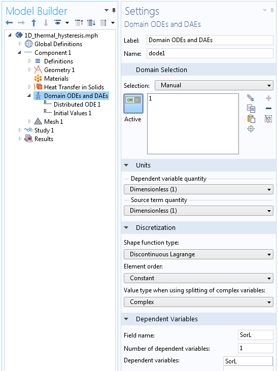
Settings for the Domain ODEs and DAEs interface that tracks the material state.
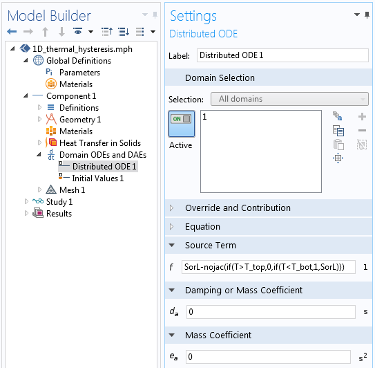
The Source Term settings.
The above screenshot depicts the equation that is being solved for in the Domain ODEs and DAEs interface. Let’s examine in detail the Source Term equation used:
SorL-nojac(if(T> T_top,0,if(T< T_bot,1,SorL)))
This equation is evaluated at the centroid of each element and implements in a single line the following:
If the current temperature is greater than the temperature of complete melting (the nominal melting temperature plus half the smoothing temperature), then the material has passed its solid-to-liquid phase-change temperature, so set SorL = 0. This means that the liquid-to-solid enthalpy curve is followed. If the current temperature is less than the temperature of complete solidification (the nominal freezing temperature minus half the smoothing temperature), then the material has passed its liquid-to-solid phase-change temperature, so set SorL = 1. This means that the solid-to-liquid enthalpy curve is followed. Otherwise, when neither of the previous two conditions are satisfied, leave the SorL variable at its previous value, meaning that there is no change of path while in the intermediate zone.
The nojac() operator tells the software to exclude the enclosed expression from the Jacobian computation, thus it does not try to differentiate the enclosed expression but merely evaluates the expression itself at each time step.
The SorL variable is used in one place in the model: in the definition of the specific heat in the phase-change material domain, as shown earlier. It is also important to set the initial value of the variable appropriately. If the initial temperature of the phase-change material is above or below the temperature of complete melting or solidification, then this choice is unambiguous; otherwise, you must choose the initial state of the material. In the example here, we will consider the initial temperature of the system to be below the freezing temperature, so the material will initially follow the solid-to-liquid path. Therefore, the initial value of the SorL variable is set to one.
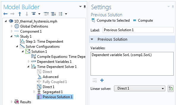
The solver settings showing the usage of the Previous Solution operator.
In terms of solving the model, we only need to keep in mind that the SorL variable needs to be evaluated at the previous time step using the Previous Solution operator in the solver sequence, as shown in the screenshot above. We can also use a segregated solver and, of course, we should investigate tightening the time-dependent solver tolerances, the scaling of the dependent variables, and study the convergence of the solution with mesh refinement.
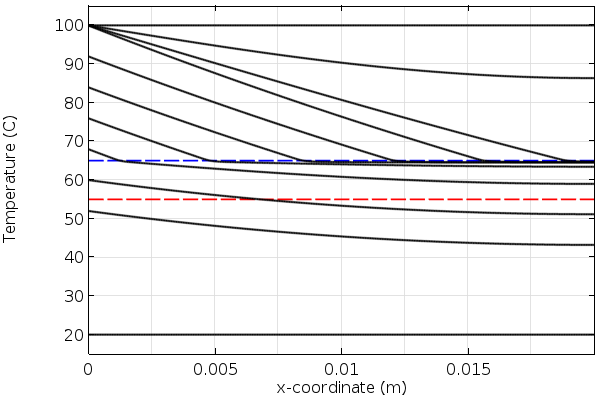
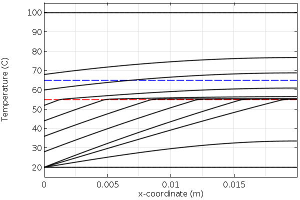
Let’s now look at some results. In the plots below, we see the temperature through the thickness of our modeling domain for the heating and cooling of the phase-change material. Observe that the slope of the temperature as a function of position changes as the material passes through the melting and freezing points. This is due to extra heat that must be added or removed as the material changes phase.
Temperature over time in the phase-change material during heating. The blue line is the melting temperature.
Temperature over time in the material during cooling. The red line is the freezing temperature.
An animation showing the combined temperature profile over time during heating and cooling. The blue and red lines are the melting and freezing temperatures.
Closing Remarks on Modeling Materials with Thermal Hysteresis
Today, we have introduced an approach appropriate for modeling materials exhibiting thermal hysteresis under the assumption of constant density and that the material must go completely above and below the melting and freezing temperatures to change phase. This modeling approach makes use of the Previous Solution operator and equation-based modeling. For more details on the usage of the Previous Solution operator and further examples, please see:
- Using the Previous Solution Operator in Transient Modeling
- Tracking Material Damage with the Previous Solution Operator
The approach shown here is a bit simplified for the sake of explanation. If you are interested in the modeling of heat transfer with phase change, either with or without hysteresis, we recommend that you look to the Heat Transfer Module, which has a built-in interface for modeling heat transfer with phase change, as introduced here.
If you are instead interested in the modeling of irreversible changes in phase, then you may also want to take a look at our previous blog post on thermal curing as well as tracking material damage with the Previous Solution operator.
Looking to model thermal hysteresis in COMSOL Multiphysics or have other questions about this process? Please contact us.


Comments (10)
A.W.M. van Schijndel
March 30, 2016Dear Walter,
This is a very good example on how to model hysteresis. Thanks! Also the procedure is quite clear. I will start to model it from scratch as explained above so I can learn how to do it.
Still one question: Is the corresponding mph model available for the users?
Kind regards
Jos van Schijndel
Walter Frei
April 1, 2016 COMSOL EmployeeDear Jos, Thank you for your feedback. If you do run into any issues following these instructions, please contact your COMSOL Support Team and we will be happy to assist.
valery vv
April 25, 2016Dear Walter Frei.
Thank you for your article.
Do you have a mph model for a more detailed study
of melting and crystallization processes?
Tom Caltabellotta
May 2, 2016Thank you Walter, this article was most informative.
Timo Herdlitschka
April 6, 2017Dear Walter,
Thank you for this article.
I just have on question, how can SorL get 1?
Best regards,
Timo Herdlitschka
Timo Herdlitschka
April 6, 2017I meant, how can get SorL smaller than 0 or bigger than 1?
Caty Fairclough
May 3, 2017Hi Timo,
Thanks for your comment!
For questions related to your modeling, please contact our Support team.
Online Support Center: https://www.comsol.com/support
Email: support@comsol.com
Sam Adu-Amankwah
July 9, 2019Hi,
Can you please add details/screen shots of the analytic functions for enthalpy and boundary temperature? Is the mph file available for version 5.3a?
Your help will be appreciated.
best regards,
Sam
Cory Cress
October 2, 2020Dear Walter,
I plotted the SorL vs x at various times. In general, the values are 0,1 as expected. However, as the phase changes, there are SorL values between 0 and 1 or even greater than 1. How is that even possible? Is it related to the discretization method for the ODE and the heat transfer not being the same?
Walter Frei
January 12, 2022 COMSOL EmployeeHello,
For an alternative approach to modeling of hysteresis, see also:
https://www.comsol.com/blogs/how-to-use-state-variables-in-comsol-multiphysics/
Note that there is also an updated file, for 6.0, and showing both methods, here:
https://www.comsol.com/model/modeling-phase-change-with-hysteresis-46801