Microfluidics Module
Perform Multiphysics Simulations of Microfluidic Devices with the Microfluidics Module

An ink droplet is ejected through a nozzle and travels through air until it hits the target. The model can be used to understand the effect of the ink properties and the pressure profile at the nozzle on the drop velocity, drop volume, and the presence of satellite drops.
General-Purpose Microfluidics Simulations
The Microfluidics Module brings you easily-operated tools for studying microfluidic devices. Important applications include simulations of lab-on-a-chip devices, digital microfluidics, electrokinetic and magnetokinetic devices, and inkjets. The Microfluidics Module includes ready-to-use user interfaces and simulation tools, so called physics interfaces, for single-phase flow, porous media flow, two-phase flow, and transport phenomena.
Scaling Down to Microscale Flows
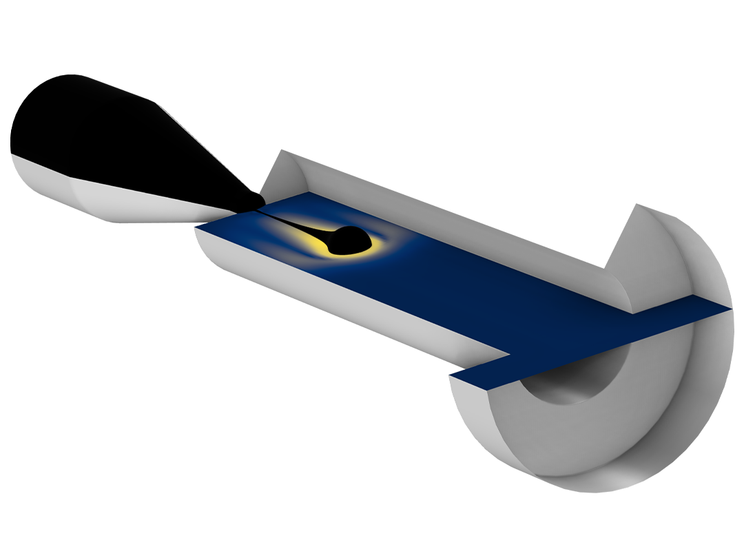
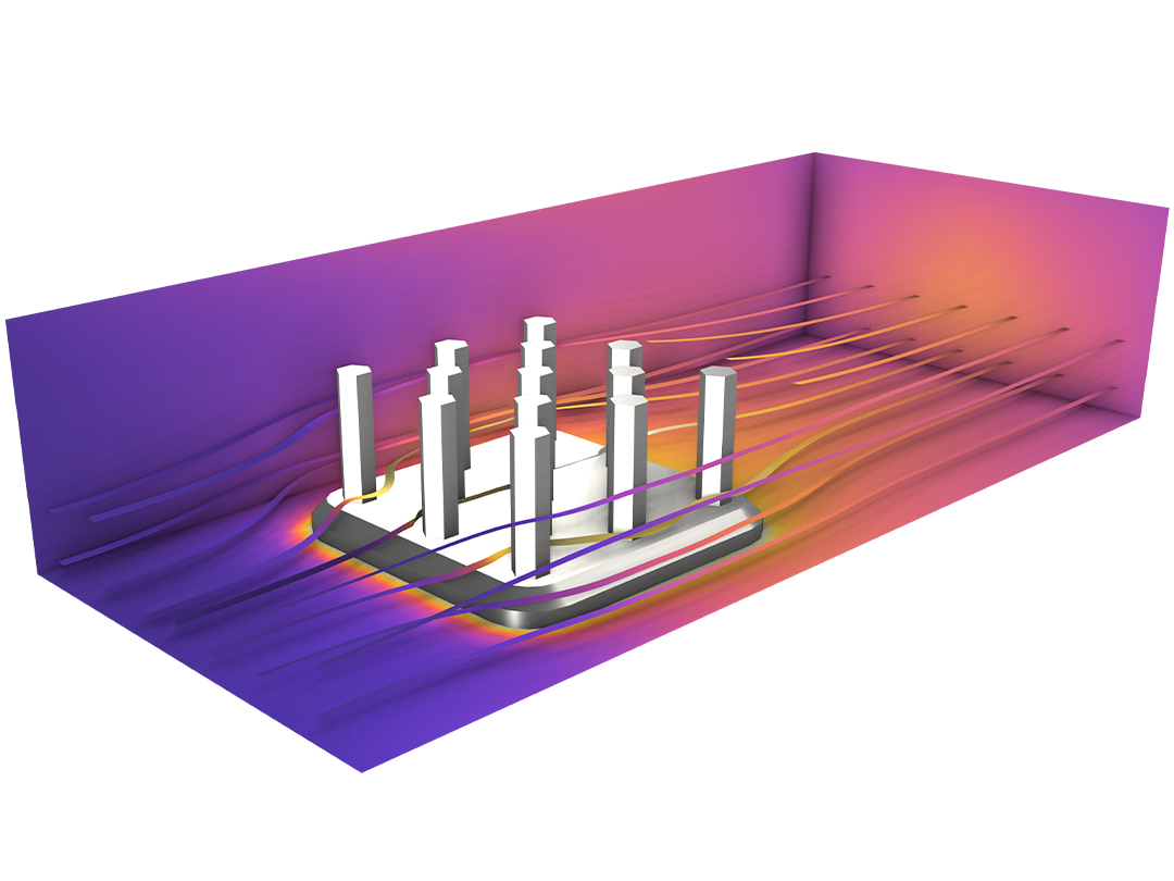
Microfluidic flows occur on length scales that are orders of magnitude smaller than macroscopic flows. Manipulation of fluids at the microscale has a number of advantages – typically microfluidic systems are smaller, operate faster, and require less fluid than their macroscopic equivalents.
Energy inputs and outputs are also easier to control (for example, heat generated in a chemical reaction) because the surface-to-area volume ratio of the system is much greater than that of a macroscopic system. In general, as the length scale of the fluid flow is reduced, properties that scale with the surface area of the system become comparatively more important than those that scale with the volume of the flow.
This is apparent in the fluid flow itself as the viscous forces, which are generated by shear over the isovelocity surfaces, dominate over the inertial forces. The Reynolds number (Re) that characterizes the ratio of these two forces is typically low, so the flow is usually laminar. In many cases, the creeping (Stokes) flow regime applies (Re«1). Laminar and creeping flows make mixing particularly difficult, so mass transport is often diffusion limited, but even in microfluidic systems diffusion is often a slow process. This has implications for chemical transport within microfluidic systems. The Microfluidics Module is designed specifically for handling momentum, heat, and mass transport with special considerations for fluid flow at the microscale.
Additional Images:


COMSOL’s general-purpose multiphysics features are uniquely suited for handling the many microscale effects that are utilized in microfluidic devices. It is easy to set up coupled electrokinetic and magnetodynamic simulations – including electrophoresis, magnetophoresis, dielectrophoresis, electroosmosis, and electrowetting. In addition, chemical diffusion and reactions for dilute species functionality included in the module enable you to simulate processes occurring in lab-on-a-chip devices. For simulating rarefied gas flows, you can use the specialized boundary conditions that activate flow simulation in the slip flow regime. The Microfluidics Module also provides dedicated methods for simulation of two-phase flow with the level set, phase field, and moving mesh methods. For each of these, the capabilities of the Microfluidics Module include surface tension forces, capillary forces, and Marangoni effects.
Workflow for Modeling Microfluidic Devices
To model a microfluidic device, you begin by defining the geometry in the software by importing a CAD file or via the geometry modeling tools that are built into COMSOL Multiphysics. For importing geometry models, several choices are available to you: the CAD Import Module, for import of mechanical CAD models; the ECAD Import Module for import of electronic layouts; and the LiveLink™ products for CAD for a direct link to models created in a dedicated CAD software package. In the next step, you select appropriate fluid properties and choose a suitable physics interface. Initial conditions and boundary conditions are set up within the interface. Next, you define the mesh. In many cases, COMSOL’s automatically created default mesh, which is produced from physics-dependent defaults, will be appropriate for the problem. A solver is selected, again with defaults appropriate for the relevant physics, and the problem is solved. Finally, you can visualize the results.You access all of these steps from the COMSOL Desktop®. The Microfluidics Module can solve for stationary and time-dependent flows in 2D and 3D, and can be coupled with any other add-on products for further extension of the modeling capabilities. One such example is for tracking particles released in the flow stream, which is made possible by combining with the Particle Tracing Module.
Single-Phase Flow
The Fluid Flow interfaces use physical quantities, such as pressure and flow rate, and physical properties, like viscosity and density, to define a fluid-flow problem. The physics interface for laminar flow covers incompressible and weakly compressible flows. This Fluid Flow interface also allows for simulation of non-Newtonian fluid flow. A physics interface for creeping flow is used when the Reynolds number is significantly less than 1. This is often referred to as Stokes flow and is appropriate for use when viscous flow is dominant. It is usually applicable to microfluidic devices.
Two-Phase Flow
Three different methods are available for two-phase flow: level-set, phase-field, and moving mesh methods. These are used to model two fluids separated by a fluid interface and where the moving interface is tracked in detail, including surface curvature and surface tension forces. The level-set and phase-field methods use a fixed background mesh and solve additional equations to track the interface location. The moving mesh method solves the flow equations on a moving mesh with boundary conditions to represent the fluid interface. In this case, additional equations are solved for the mesh deformation by means of the arbitrary Lagrangian-Eulerian (ALE) method. All of these methods and their physics interfaces support both compressible and incompressible laminar flows, where one or both fluids can be non-Newtonian.
Rarefied Flow
Rarefied gas flow occurs when the mean free path of the molecules becomes comparable with the length scale of the flow. The Knudsen number, Kn, characterizes the importance of rarefaction effects on the flow. As the gas becomes rarefied (corresponding to increasing Knudsen number), the Knudsen layer, which is present within one mean free path of the wall, begins to have a significant effect on the flow. For Knudsen numbers below 0.01, rarefaction can be neglected and the laminar flow physics interfaces of the Microfluidics Module can be used with non-slip boundary conditions. For slightly rarefied gases (0.01<Kn<0.1), the Knudsen layer can be modeled by appropriate boundary conditions at the walls together with the continuum Navier-Stokes equations in the domain. In this instance, a special Slip Flow physics interface is available in the Microfluidics Module. To model higher Knudsen numbers, the Molecular Flow Module is required.
Porous Media Flow
Flow through porous media can also occur on microscale geometries. The flow is often friction-dominated when the pore size is in the micron range and Darcy’s law can be used. The Microfluidics Module features a dedicated physics interface for porous media flow based on Darcy's law. In this case, shear stresses perpendicular to the flow are neglected. For intermediate flows, a physics interface for the Brinkman equations is available. This physics interface models flow through a porous medium where shear stresses cannot be neglected. Both the Stokes-Brinkman formulation, suitable for very low flow velocities, and Forchheimer drag, which is used to account for effects at higher velocities, are supported. The fluid can be either incompressible or compressible, provided that the Mach number is less than 0.3.
A special physics interface for free and porous media models, both porous media using the Brinkman equations and laminar flow, automatically providing the coupling between the two. These interfaces are appropriate for microfluidic porous media flow. Example applications include paper microfluidics and transport in biological tissue.
Electrohydrodynamics Effects
At the microscale, a range of electrohydrodynamic effects can be exploited to influence the fluid flow. The Microfluidics Module is an excellent tool for modeling virtually any such effect. The electric field strength for a given applied voltage scales beneficially, making it easier to apply relatively large fields to the fluid with moderate voltages. In electroosmosis, the uncompensated ions in the charged electric double layer (EDL) present on the fluid surfaces are moved by an electric field, causing a net fluid flow. The Microfluidics Module provides a specialized electroosmotic velocity boundary condition as one of several fluid wall boundary conditions. Electrophoretic and dielectrophoretic forces on charged or polarized particles in the fluid can be used to induce particle motion, as can diamagnetic forces in the case of magnetophoresis. The Particle Tracing Module provides ready-to-use electrophoretic and dielectrophoretic particle forces. Combining the Microfluidics Module with the AC/DC Module enables you to model AC dielectrophoresis.
The manipulation of contact angles by the electrowetting phenomena is also easy in microscale devices. Electrowetting is a phenomenon that has been exploited as a basis for various new display technologies. The Microfluidics Module allows for direct manipulation of the contact angle with user-defined expressions including voltage parameters.
Mass Transport
The Microfluidics Module provides a dedicated physics interface for transport of diluted species. It is used to simulate chemical species transport through diffusion, convection (when coupled to fluid flow), and migration in electric fields for mixtures where one component – a solvent – is present in excess (90 mol% or greater). It is typically employed to model the performance of mixers. For modeling chemical reactions in microfluidic devices, you can combine the Microfluidics Module with the Chemical Reaction Engineering Module, which also makes available transport of concentrated species with binary diffusion.
Flexible and Robust Microfluidics Simulation Platform
For each of the Microfluidics interfaces, the underlying physical principles are expressed in the form of partial differential equations, together with corresponding initial and boundary conditions. COMSOL’s design emphasizes the physics by providing you with the equations solved by each feature and offering you full access to the underlying equation system. There is also tremendous flexibility to add user-defined equations and expressions to the system. For example, to model the transport of a species that significantly affects the viscosity of the fluid, simply type in concentration-dependent viscosity – no scripting or coding is required. When COMSOL compiles the equations, the complex couplings generated by these user-defined expressions are automatically included in the equation system. The equations are then solved using the finite element method and a range of industrial-strength solvers. Once a solution is obtained, a vast range of postprocessing tools are available to interrogate the data, and predefined plots are automatically generated to show the device response. COMSOL offers the flexibility to evaluate a wide range of physical quantities, including predefined quantities such as the pressure, velocity, shear rate, or the vorticity (available through easy-to-use menus), and arbitrary user-defined expressions
Interfacing with Excel® and MATLAB®
You can combine the Microfluidics Module with Microsoft Excel® via LiveLink™ for Excel®. This LiveLink™ product adds a COMSOL tab and specialized toolbar to the Excel ribbon for controlling the parameters, variables, and mesh, or for running a simulation. It also includes the capability to import and export Excel files for parameter and variable lists in the COMSOL Desktop®.
If you wish to drive COMSOL simulations by means of script programming, you can use MATLAB® and COMSOL together through the interface provided by the LiveLink™ for MATLAB®. With this LiveLink™, you can access all the functionality of the COMSOL Desktop® from a wealth of MATLAB commands. This provides a programmatic alternative to using the COMSOL Desktop® for microfluidics simulations.
Product Features
- Anisotropic porous media flow
- Arbitrary user-defined expression for postprocessing
- Automatic boundary layer meshing
- Built-in variables for computing the Reynolds, Prandtl, Nusselt, Rayleigh, and Grashof numbers
- Creeping flow
- Capillary forces
- Electrokinetic effects
- Flow in porous media through Darcy's Law and the Brinkman Equations
- Fluid-structure interaction (FSI)1
- Forchheimer drag for porous media flow
- Laminar flow
- Marangoni effects
- Migration effects
- Multiple species user interface
- Newtonian and non-Newtonian flow
- Particle tracing methods where particles can affect the flow (Lagrange-Euler)2
- Slip flow
- Shallow channel approximation for 2D flow
- Species transport in porous media
- Surface tension effects
- Two-phase flow with the Level-set method
- Two-phase flow with the phase-field method
- Two-phase flow with the moving mesh method based on an arbitrary Lagrangian-Eulerian (ALE) formulation
- Part Library with parametric geometry parts for channels in microfluidic components representing common configurations
1 Together with the Structural Mechanics Module or MEMS Module
2 Together with the Particle Tracing Module
Application Areas
- Capillary devices
- Chemical and biochemical sensors
- Dielectrophoresis (DEP)
- DNA chips
- Electrocoalescence
- Electrokinetic flow
- Electroosmosis
- Electroosmosis
- Electrowetting
- Emulsions
- Inkjets
- Lab-on-a-chip
- Magnetophoresis
- Microreactors, micropumps, and micromixers
- Microfluidic sensors
- Slightly rarefied gas flow (slip flow)
- Static mixers
- Surface tension effects
- Two-phase flow
- Polymer flow and viscoelastic flow
- Optofluidics
Droplet Breakup in a T-Junction
Emulsions consist of small liquid droplets immersed in an immiscible liquid and widely occur in the production of food, cosmetics, fine chemicals, and pharmaceutical products. The quality of the product is typically dependent on the size of the droplets. Simulating these processes can help in optimizing these droplets as well as other process ...
Capillary Filling
This example studies a narrow vertical cylinder placed on top of a reservoir filled with water. Because of wall adhesion and surface tension at the air/water interface, water rises through the channel. Surface tension and wall adhesive forces are often used to transport fluid through microchannels in MEMS devices or to measure, transport and ...
Separation Through Electrocoalescence
Applying an electric field across a suspension of immiscible liquids may stimulate droplets of the same phase to coalesce. The method known as electrocoalescence has important applications, for instance, in the separation of oil from water. To model electrocoalescence, you need to solve the Navier-Stokes equations, describing the fluid motion, ...
Inkjet Nozzle — Level Set Method
Although initially invented to be used in printers, inkjets have been adopted for other application areas, such as within the life sciences and microelectronics. Simulations can be useful to improve the understanding of the fluid flow and to predict the optimal design of an inkjet for a specific application. The purpose of this application is to ...
Transport in an Electrokinetic Valve
This application presents an example of pressure driven flow and electrophoresis in a 3D micro channel system. Researchers often use a device similar to the one in this model as an electrokinetic sample injector in biochips to obtain well-defined sample volumes of dissociated acids and salts and to transport these volumes. Focusing is obtained ...
Drug Delivery System
This example describes the operation of a drug delivery system that supplies a variable concentration of a water soluble drug. A droplet with a fixed volume of water travels down a capillary tube at a constant velocity. Part of the capillary wall consists of a permeable membrane separating the interior of the capillary from a concentrated ...
Electrowetting Lens
The contact angle of a two-fluid interface with a solid surface is determined by the balance of the forces at the contact point. In electrowetting the balance of forces at the contact point is modified by the application of a voltage between a conducting fluid and the solid surface. In many applications the solid surface consists of a thin ...
Controlled Diffusion Separator
This model simulates an H-shaped micro-cell designed for diffusion-controlled separation. The cell puts two different laminar streams in contact for a controlled period of time. The contact surface is well-defined and, by controlling the flow rate, it is possible to control the amount of species that are transported from one stream to the other ...
Lamella Mixer
At the macroscopic level, systems usually mix fluids using mechanical actuators or turbulent 3D flow. At the microscale level, however, neither of these approaches is practical or even possible. This model demonstrates the mixing of fluids using laminar-layered flow in a MEMS mixer. This model analyzes the steady-state condition of the fluid ...
Electroosmotic Micromixer
Microlaboratories for biochemical applications often require rapid mixing of different fluid streams. At the microscale, flow is usually highly ordered laminar flow, and the lack of turbulence makes diffusion the primary mechanism for mixing. While diffusional mixing of small molecules (and therefore of rapidly diffusing species) can occur in a ...
Every business and every simulation need is different.
In order to fully evaluate whether or not the COMSOL Multiphysics® software will meet your requirements, you need to contact us. By talking to one of our sales representatives, you will get personalized recommendations and fully documented examples to help you get the most out of your evaluation and guide you to choose the best license option to suit your needs.
Just click on the "Contact COMSOL" button, fill in your contact details and any specific comments or questions, and submit. You will receive a response from a sales representative within one business day.
Next Step
Request a Software Demonstration