We’ve learned how to simulate a simple bit-by-bit holographic data storage model in COMSOL Multiphysics by choosing an appropriate beam size and implementing the recording and retrieval process. Today, we step forward and demonstrate how to simulate a more difficult and complex, yet more realistic and interesting model of a holographic page data storage system.
Designing a Simulation for a Holographic Page Data Storage System
In a previous blog post discussing bit-by-bit hologram simulation, we introduced holographic data storage, its applications in consumer electronics, and how to simulate a bit-by-bit hologram. Now, we’ll discuss the other form of holographic data storage: page data storage. A page is a block of data represented by a spatial light modulator (SLM) that is either transmissive or reflective by using microelectromechanical systems (MEMS) or liquid crystal on silicon (LCoS).
As mentioned in the previous blog post, simulation for holographic data storage has traditionally been performed by the beam propagation method, which can handle very large computational domains, but cannot correctly handle a large focusing angle. COMSOL Multiphysics, on the other hand, uses a full-wave method, which can handle any kind of beam, but uses relatively more memory. With COMSOL Multiphysics, we can simulate a page (multibyte) data storage system in a small domain. To demonstrate, let’s consider a rectangular domain similar to that used in the previous study. This time, we will cipher one-byte (or eight bits) of data.
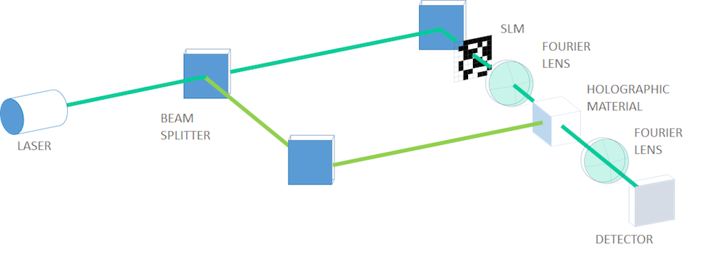
A typical optical layout of page-type holographic data storage (the character code of my name is encoded in binary data in the SLM).
For this simulation, we will use the binary data converted from the character code of a part of my own name in its native language. 01001101, which means “water”, can be seen in the fifth row in the SLM in the image above. To be more realistic, we’ll use a set of Fourier lenses to focus the object beam into the holographic material to record, expand, and visualize the retrieved object beam onto the detector in the retrieval process. Of course, we won’t model a lens, but instead make a focused beam by Fourier transforming the electric field amplitude after the SLM and providing it as the incident field in the scattering boundary condition on the incident boundary.
To image the retrieved object beam on the detector, we again Fourier transform the retrieved electric field amplitude and square the norm to get an intensity that a charge-coupled device (CCD) or complementary metal-oxide semiconductor (CMOS) sensor detects as a signal. More signal processing takes place afterward to create a cleaner signal and lessen the bit error rate to a significantly smaller level, but we will not go into this process here.
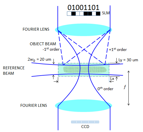
A holographic page data storage system, carrying one-byte data.
Defining the Reference Beam
In our previous discussion, we used a slightly diverging super Gaussian beam. For this simulation, the domain size will be inevitably wider along the direction of the reference beam propagation, which we will discuss later. So, if we use a diverging beam, the beam will eventually touch the boundaries, which needs to be avoided. Instead of launching a 10 um beam with a flat phase on the left boundary, we will add the following quadratic phase function so the beam slightly focuses in the middle of the domain, assuming the out-of-plane electric field solved for
where w_r is the waist radius of the reference beam, n is the refractive index of the holographic material, k_0 is the wave number in the vacuum, and R_r is the wavefront curvature at distance x from the beam waist (focal plane) position defined by
Here, x_R=n \pi w_r^2/\lambda_0 is the Rayleigh range in which the beam is almost straight.
For w_r = 10 um, \lambda_0 = 1 um, and n = 1.35, it gives x_R = 424 um. We will see later that this number is far larger than our domain size, which means that the beam is almost collimated in the computational domain. To define the wavefront curvature, we have borrowed the paraxial Gaussian beam formula. We ignored a constant phase and the Gouy phase, which are not necessary here. The image below shows how to enter the incident field with a right curvature at the left boundary (x=-L_x/2).
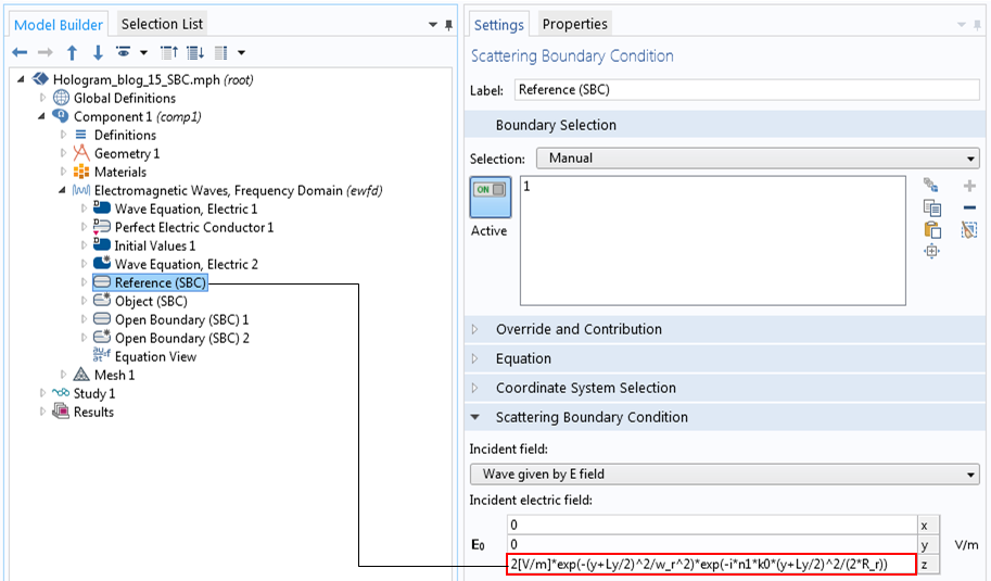
Defining the reference beam with a wavefront curvature.
Defining the Object Beam
As we are using a 10 um beam radius, the vertical domain size, L_y, of 30 um is large enough. The biggest obstacle here is how to determine the horizontal domain size, L_x, for the object beam entrance. Now, the aperture through which the object beam transmits is a 1 x 8 SLM with 8 pixels. The SLM behaves like a diffraction grating with a period of 2d. When the object beam transmits through the SLM and is focused, the zeroth-order beam is focused into a circle of the so-called Airy ring radius and the diffracted beams of higher orders will spread out at angles corresponding to the diffraction orders.
To get sufficient information from the SLM and store correct data in the holographic material, we want to capture up to at least the first-order beams (0th and ±1st). Otherwise, we may get some retrieved signal, but the signal might not fully restore the original data. Another reason why we only take up to the first orders is because all other higher orders will be too weak in intensity to be recorded in the holographic material.
The first requirement is that the zeroth-order beam radius, w_0, must be 10 um, which determines the numerical aperture (NA) of the lens system. The Airy ring radius, w_0, is given by the Airy ring radius formula
where \lambda_0 is the wavelength in the air.
We want the Airy ring radius to be 10 um. From this requirement, we get the NA for a given w_0 and \lambda_0 as
On the other hand, the NA is originally defined as
where \theta is the focusing angle, N is the number of SLM pixels, d is the half size of the SML pixel, and f is the focal length of the Fourier lens.
From this equation, a ratio, f/d, is derived as
We apply the grating equation for the first order
where \alpha_1 is the diffraction angle of the first-order beams.
We get the deviation w_1 of the beam position of the first-order beams from the zeroth-order beam at a distance f as
Inserting the known numbers, N = 8 and w_0 = 10 um, we get w_1 = 65.6 um. Adding some margin to capture the “whole” first-order beams, half of L_x may be 80 um; that is, L_x = 160 um. It’s worth mentioning that this particular figure is one of the key elements of holographic technology.
Other than this number, \lambda_0, f, and d are undetermined. Now that we know all of the domain sizes, we can estimate the number of meshes needed from the maximum mesh size, \lambda_0/6/(2n\sin(\beta/2)) = \lambda_0/(6\sqrt{2}n), where n is the refractive index of the holographic material and \beta is the intersecting angle between the object and reference beams. With the RAM capacity of my own computer, \lambda_0 = 1 um seems to be the shortest wavelength. Then, we get f/d = 131.1, of which the numbers f and d are dependent. For now, let d be 40 um, followed by f = 5.2 mm. We now have all of the simulation parameters.
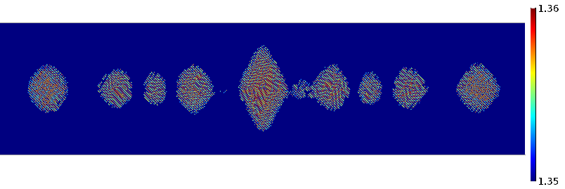
To prepare the 1 x 8 pixel data, we can define the primitive built-in rectangular function to represent a single pixel. To make pixel data, the rectangular function is shifted and added up. 01001101 is defined as an analytic function, as shown in the figure below. The open subapertures stand for “1”.
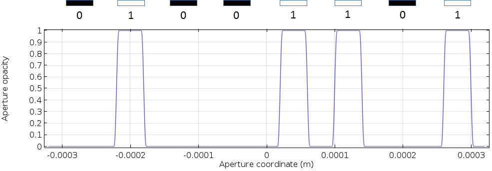
An SLM aperture opacity function, representing the eight-bit data of 01001101.
Implementing a Fourier Transformation in COMSOL Multiphysics
Next, we focus the object beam. In Fourier optics, the image of the input electric field that is focused by a Fourier lens in the focal plane is the Fourier transform of the input field. The complex electric field amplitude in the image plane focused by a Fourier lens with the focal length f is calculated by
where u is the spatial coordinate in the Fourier/image space and u/(f\lambda_0) represents the spatial frequency.
Do we need to use additional software to implement the Fourier transformation? No. By using COMSOL Multiphysics, all of the required capabilities are included in one package. You can also use COMSOL Multiphysics as a convenient scientific computational software in the GUI of the same platform as other finite element computations.
The Settings window is shown in the figure below, followed by the result of the Fourier transformation of the page data 01001101, calculated by the COMSOL software.
The settings for the incident object beam, which is the Fourier transform of the electric field amplitude after the SLM.
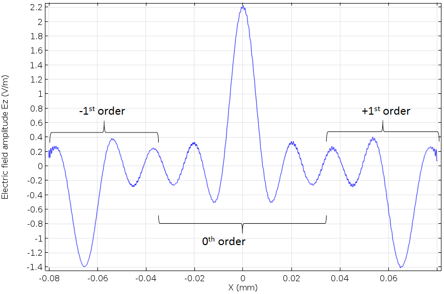
The computed incident object beam as the Fourier transform of the binary data 01001101.
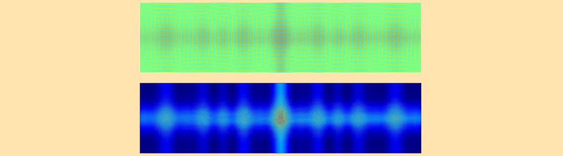
The center beam is the zeroth-order beam and the two side beams with the opposite phase are the first-order beams. This is a typical Fraunhofer diffraction pattern of a grating. As we calculated before, our computational domain fits these three beams exactly. This electric field amplitude is given as the Electric Field boundary condition for the object beam. The following figures are the result of the page data recording.
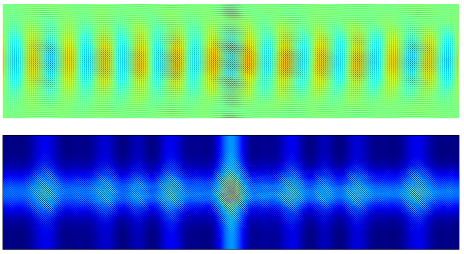
The electric field amplitude (top) and intensity (bottom) for the page data recording.
Our hologram simulation is starting to look more interesting thanks to our encoding and ciphering work. The data for my name has been encoded by an industrial standard and then converted to a binary code. Then, it was Fourier transformed by a Fourier lens, which can be thought of as another ciphering process. Finally, the code was ciphered in a hologram. Of course, you can’t crack the code by simply looking at any of the images above.
Retrieving the Holographic Data
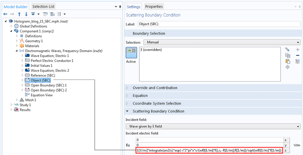
Next, we move on to the data retrieval step. To retrieve the data, as was described in the previous blog post, we can use the same COMSOL Multiphysics feature to turn the functionalities on and off. We do this by adding the Wave Equation, Electric 2 node with a user-defined refractive index, which specifies the modulated index.
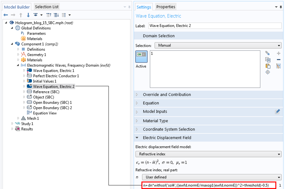
The Settings window for the modulated refractive index.
The modulated refractive index. The modulation amplitude corresponds to the position where the electric field intensity exceeds the threshold.
By turning the object beam off and keeping the reference beam on, as well as having the modulated index, we get the result of the retrieval simulation.
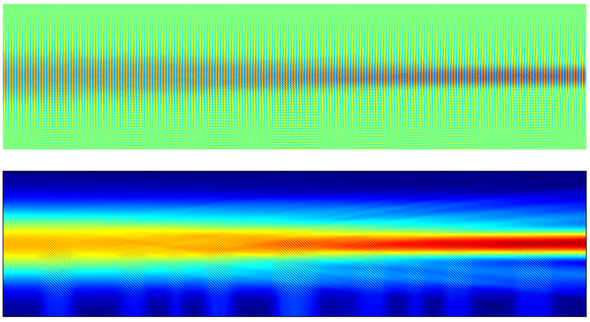
The electric field amplitude (top) and intensity (bottom) for the page data retrieval.
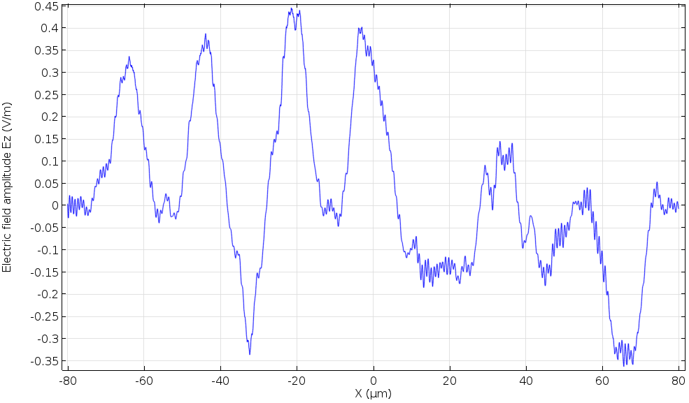
The electric field amplitude at the bottom edge during page data retrieval (cross section).
Now, we want to image this retrieved data onto the CCD surface by using the other Fourier lens. To do so, we will Fourier transform the retrieved electric field amplitude again and take the square of this amount. The following figure is the final result. The CCD detects the 1 positions in the original code, 01001101. We finally see the code again!
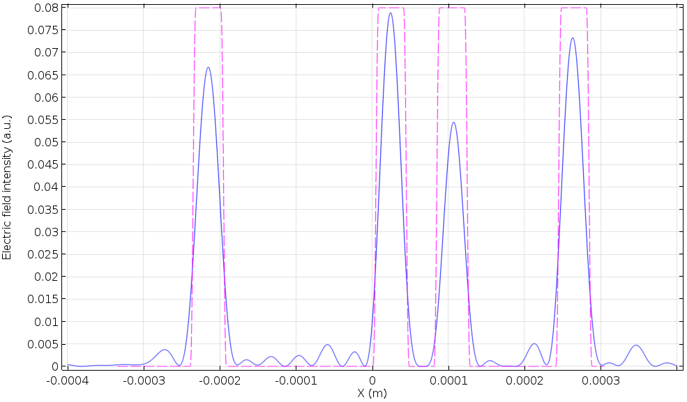
The retrieved data on the CCD surface. The dashed line represents the position of 1 in the original code.
Concluding Remarks on Holographic Page Data Storage
We have implemented a holographic page data storage model using the wave optics capabilities of COMSOL Multiphysics. Though the rigorous Maxwell solver persuades us to pay more attention to some specific restrictions, we were able to catch a glimpse of the holography created by the design calculation we performed prior to the simulation. We also went over some helpful and convenient uses of COMSOL Multiphysics as a scientific calculator. As we learned, the COMSOL software can perform all of these tasks in one environment, with sequential finite element computations and other scientific calculations performed simultaneously.
Further Reading
- Check out the COMSOL Blog:
- Take a look at the first part of this series for an introduction to holographic data storage
- Read about the built-in integration operators for the Fourier transformation
- Learn more about Fourier optics with the book Introduction to Fourier Optics by J.W. Goodman


Comments (8)
Ivan Stoloka
April 7, 2018Hello, looks great, is there a possibility to download model file?
Thanks.
Yosuke Mizuyama
April 9, 2018 COMSOL EmployeeDear Ivan,
Thank you for reading the blog.
We will try to provide you with the model file.
Best regards,
Yosuke
Ferdous Anik
August 12, 2018Can get the model file of earliar version(5.3.0.260)
Yosuke Mizuyama
August 13, 2018 COMSOL EmployeeHi Ferdous,
Thank you for reading my blog. Could you please send the request to support@comsol.com?
Thank you!
Best regards,
Yosuke
Eunso Shin
June 25, 2020Hi Yosuke, thanks for sharing.
I would like to ask why you didn’t use the Gaussian beam at Electromagnetic Waves, Frequency Domain, but SBC.
What is the difference between them?
Could you explain the advantages and disadvantages of them?
Thanks a lot!
Yosuke Mizuyama
June 25, 2020 COMSOL EmployeeDear Eunso,
Thank you for reading my blog.
Do you mean the built-in Gaussian beam boundary feature?
If so, at the time I wrote this blog, we didn’t have it yet.
The difference between the field used in this blog and the built-in Gaussian beam is the Gouy phase.
For very large beam sizes, the Gouy phase is almost zero. So I didn’t include the term in the model in this blog
while the built-in Gaussian beam has it for accuracy for all beam sizes.
Best regards,
Yosuke
Xi Shen
October 17, 2023Hello, this is awesome, is there a possibility to download model file? I also wonder what is tha scale of the simulation, the thickness is 2o um, what’s the length?
Yosuke Mizuyama
October 19, 2023 COMSOL EmployeeHello Xi Shen,
Thank you for reading my blog. The size of the domain is 32×162 um^2.
Unfortunately, this model isn’t published but please try to request through
support@comsol.com.
The basic setting for this model is the same as in
https://www.comsol.com/model/single-bit-hologram-34921.
I hope this helps.
Best regards,
Yosuke