
When designing bandpass-filter type high-Q RF devices with the finite element method in the frequency domain, you will likely come across a situation where you need to apply many frequency samples to more accurately describe the passband. Simulation time is directly proportional to the number of frequencies included in the simulation of a microwave device, with the time increasing as the frequency resolution becomes finer. Two powerful simulation methods in the RF Module, an add-on to the COMSOL Multiphysics® software, help accelerate the modeling of such devices.
Editor’s note: This blog post was originally published on July 4, 2016. It has since been updated to reflect up-to-date functionality and results representation.
A Brief Introduction to the Two RF Simulation Methods
The two simulation methods that we will discuss in today’s blog post are the asymptotic waveform evaluation (AWE) and frequency-domain modal (FDM) methods. Both methods are designed to help you overcome the conventional issue of a longer simulation time when using a very fine frequency resolution or running an ultra-wideband simulation with a regular Frequency Domain study. The AWE method is quite efficient when it comes to describing smooth frequency responses with a single resonance or no resonance at all. The FDM method, meanwhile, is useful for quickly analyzing multistage filters or filters of a high number of elements that have multiple resonances in a target passband. In the next two sections, we are going to discuss their typical settings and use cases.
It’s worth mentioning that the AWE and FDM methods are both almost independent of the frequency step selected. You can decrease the value of the frequency step freely and get a well-resolved plot without any notable slowdown or extra memory consumption. However, there’s one drawback: Decreasing the value of the frequency step may affect the amount of data saved as a final solution. Later in this blog post, in the section dedicated to data management, you will find recommendations that allow for a significant reduction of output file size.
Note that before running either an AWE or FDM calculation with the fine resolution, it may be useful to perform a preliminary Eigenfrequency and regular Frequency Domain simulation with a coarse frequency resolution. This would give you a fast and valuable estimation of resonance locations and a general understanding of the system’s frequency trends, including for the actual passbands and the desired frequency resolution.
Asymptotic Waveform Evaluation Method Fosters Reduced-Order Modeling
For our purposes, it would be too technical to talk about the numerical characteristics and mathematical algorithms of AWE — an advanced reduced-order modeling technique. Instead, we will go over how to use this method in the RF Module. As of version 6.2 of COMSOL Multiphysics®, there is a dedicated Adaptive Frequency Sweep study step that implements the AWE method. When using this feature, you should specify a target output frequency range and choose an expression to be used for error estimation by the AWE algorithm. Under the hood, the solver performs fast-frequency adaptive sweeping and uses, by default, Padé approximations.
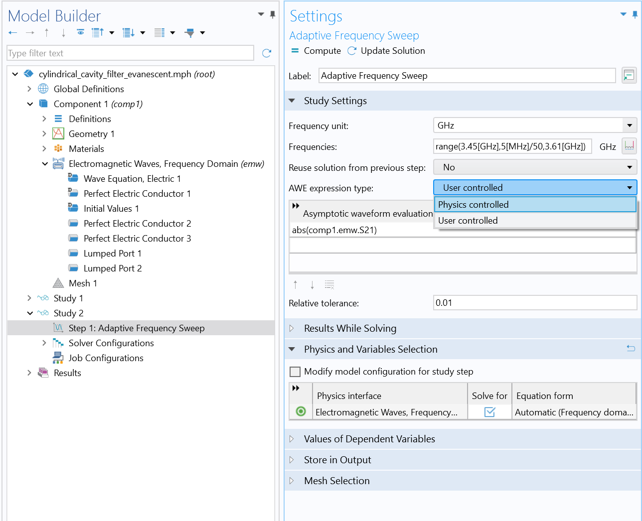
The Adaptive Frequency Sweep study settings. Check out the default Asymptotic waveform evaluation (AWE) expression used.
The AWE method is very useful when simulating resonant circuits, especially bandpass-filter type devices with many frequency points. For instance, the Evanescent Mode Cylindrical Cavity Filter tutorial model, available in the Application Library, initially sweeps the simulation frequency between 3.45 GHz and 3.61 GHz with a 5 MHz frequency step via a regular Frequency Domain study.
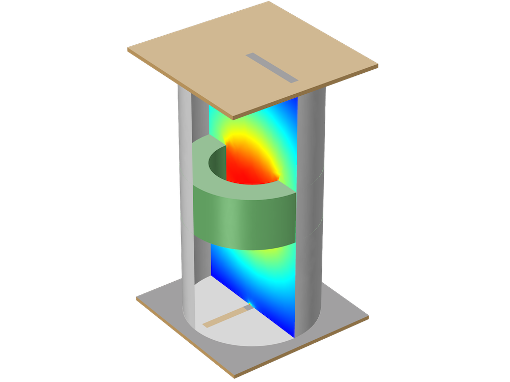
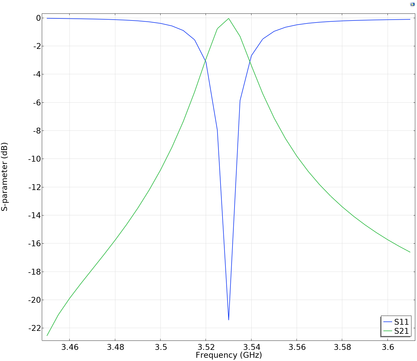
The Evanescent Mode Cylindrical Cavity Filter tutorial model (left) and its discrete frequency sweep results (right). The S-parameter plot does not look smooth around the resonant frequency.
Say you want to run the simulation again with a much finer frequency resolution, such as a 100 kHz frequency step that is 50 times finer. You can expect that the simulation will take 50 times longer to finish. But when using the Adaptive Frequency Sweep study in this particular example model, the simulation time is almost the same as the regular frequency sweep case, but we can obtain all of the computed solutions on the dependent variable with the 100 kHz frequency step.
The simulation time may vary to some extent in regard the user input in the AWE expressions. Any model variable works as an AWE expression, so long as it generates a smooth resulting plot like a Gaussian pulse or a smooth curve as a function of frequency, but the obvious and typical choice is a global expression based on S-parameters. For instance, the absolute value of S21 (abs(comp1.emw.S21)) works great as the input for the AWE expression in the case of a two-port bandpass filter. Consider that if the frequency response of the AWE expression contains an infinite gradient — the case for the S11 value of an antenna with excellent impedance matching at a single frequency point — the simulation will take longer to complete. If the loss from the antenna is negligible, an alternative expression such as sqrt(1-abs(comp1.emw.S11)^2) may work better and reduce the computation time. The aforementioned expressions are the default Physics controlled choices for the Asymptotic waveform evaluation (AWE) expression. As a sanity check, you can always run a preliminary Frequency Domain sweep with a coarse resolution, plot the expressions, and choose the smoothest one.
When you are ready to run the Adaptive Frequency Sweep don’t forget to use the desired finer frequency step in the study settings. Once the simulation is complete, you will notice that the simulation time is almost the same as the discrete sweep. Let’s compare the computed S-parameters. Since the AWE solver performed a frequency sweep that was 50 times finer, its frequency response (S-parameters) plot consequently looks much nicer. Not only do you save precious time with this approach, but as the plot below illustrates, you also still obtain accurate and good-looking results with the resonance frequency located more accurately. As a validation, the curious reader can run a regular sweep with the same resolution and check that the results are in perfect correlation.
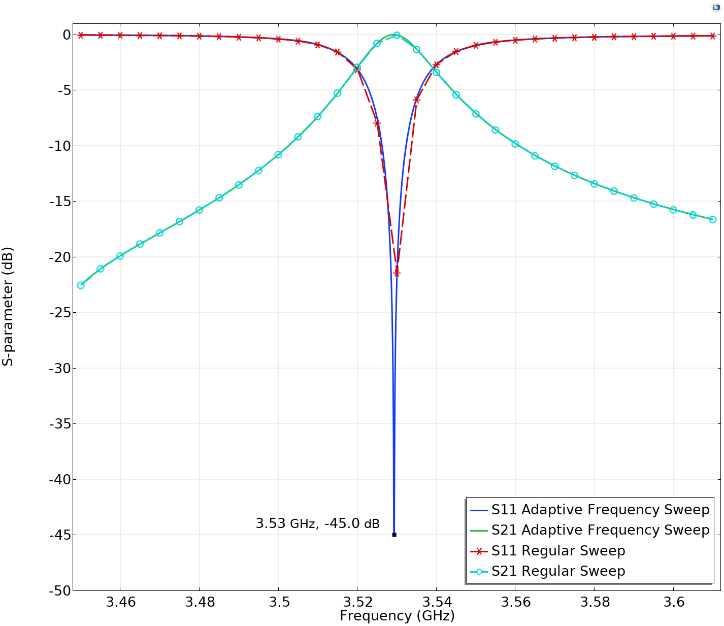 S-parameter plot resulting from the Adaptive Frequency Sweep (AWE) and discrete Frequency Domain simulations. The resolution of the AWE results is 50 times finer.
Frequency-Domain Modal Method Captures the Resonance of Circuits
Bandpass-frequency responses of a passive circuit result from a combination of multiple resonances, so the FDM method is the optimal choice for accelerating their modeling. Usually it contains two subsequent steps. The Eigenfrequency analysis is key to capturing the resonance frequencies of an arbitrary shape of a device. Once we obtain all of the necessary information from the eigenfrequency analysis, we can reuse it in the frequency-domain modal study. Doing so enables us to optimize the efficiency of the simulation when a finer frequency resolution is required to more accurately describe the frequency response, as illustrated in the AWE method.
To perform an FDM analysis seamlessly, there are a couple of aspects to keep in mind. On one hand, you need to filter out all unwanted unphysical low-frequency residues that may be present in the Eigenfrequency solution. On the other hand, you need to consider all physical modes that may affect the device’s performance in the target frequency range to get the correct results. Reaching both requirements involves some tuning of the Eigenfrequency study settings (seen in the screenshot below). First, it’s beneficial to select Larger real part as the Search method around shift setting. Next, for the Search for eigenfrequencies around setting, the lowest passband frequency works as a ballpark value. Finally, the Desired number of eigenfrequencies setting must be adjusted (based on preliminary tests, for instance) to include the necessary amount of modes.
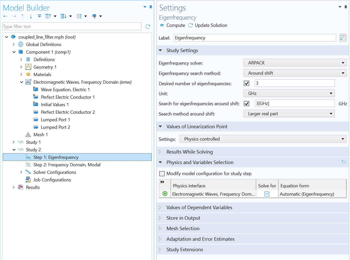 The two-step Frequency Domain, Modal study is added to the model. Here, the Eigenfrequency settings are highlighted.
To try out an FDM analysis, let’s take a look at the the Coupled Line Filter tutorial model, available in our Application Gallery. Initially, the simulation frequency sweeps between 3.00 GHz and 4.20 GHz with a 50 MHz frequency step within a regular Frequency Domain study.
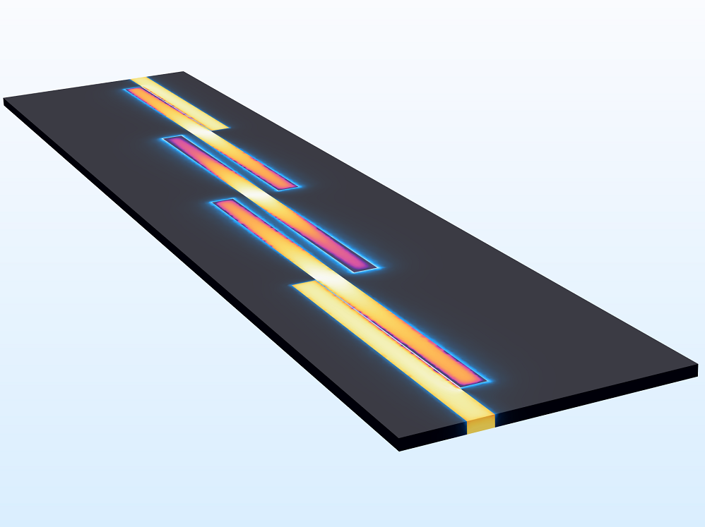
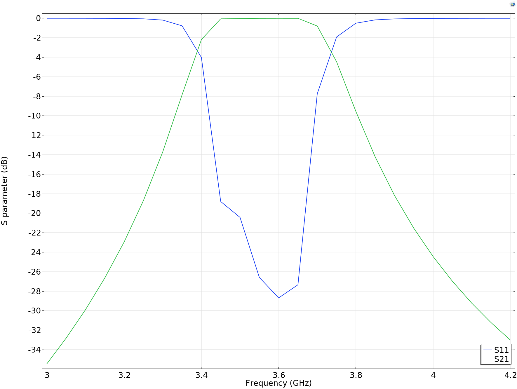
The Coupled Line Filter tutorial model (left) and its discrete frequency sweep results (right) with the resolution of 50 MHz. The S-parameter plot does not look smooth across the target passband.
Next, you can employ the Frequency Domain, Modal study, configuring the settings for each study step as described above. Run the study with the a frequency step that is 50 times finer and check the result enhancement. Just as with the AWE method, the S-parameter plot returned by the FDM study looks smoother and is more informative. For instance, it showcases all of the S11-parameter ripples that were missing initially. As a validation, the curious reader can run a regular sweep with the same resolution and check that the results are in perfect correlation.
Note that the eigenfrequency analysis contains a lumped port that impacts the simulation as an extra loading factor, so the phase of the computed S-parameters is different from that of the regular frequency sweep model. The results are compatible only with phase-independent S-parameter values such as dB-scaled, absolute value, reflectivity, or transmittivity.
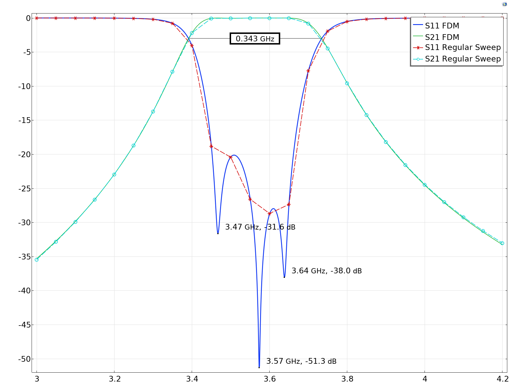
S-parameter plot resulting from the Frequency Domain, Modal (FDM) and discrete Frequency Domain simulations. The resolution of the FDM results is 50 times finer.
It’s not directly related to the original topic, but in the last figure you may notice special Graph Markers that highlight all the local minima of the S11-parameter plot as well as the passband for the S21-parameter plot. Along with the interactive result extraction from the graph plot, another recent enhancement of results evaluation functionality in COMSOL Multiphysics®, it moves the informative and interactive value of results to a new level.
Data Management When Working with Fine Frequency Resolution
As mentioned earlier, there are no real limits on how you can refine a frequency sweep with the AWE or FDM approach. However, with a really fine resolution, the solutions would contain a ton of data. As a result, the model file size will increase tremendously when saved. In most passive RF and microwave device designs, it is a common theme that only the S-parameters are of interest, and in such cases, it is not necessary to store all of the field solutions. By choosing the appropriate option under the Store in Output section of a study, we can control the part of the model on which the computed solution is saved. For example, we can only add the selection, or selections, containing the boundaries where the S-parameters are calculated. These are the boundaries assigned as Ports or Lumped Ports, and they are typically small compared to the entire modeling domain, so the total file size can be reduced dramatically.
Note that you can add such an explicit selection when setting up a port by clicking the Create Selection icon in the Boundary Selection section once the selection is specified. You can then add the needed explicit selections created from the ports under the Store in Output section of a relevant study step.
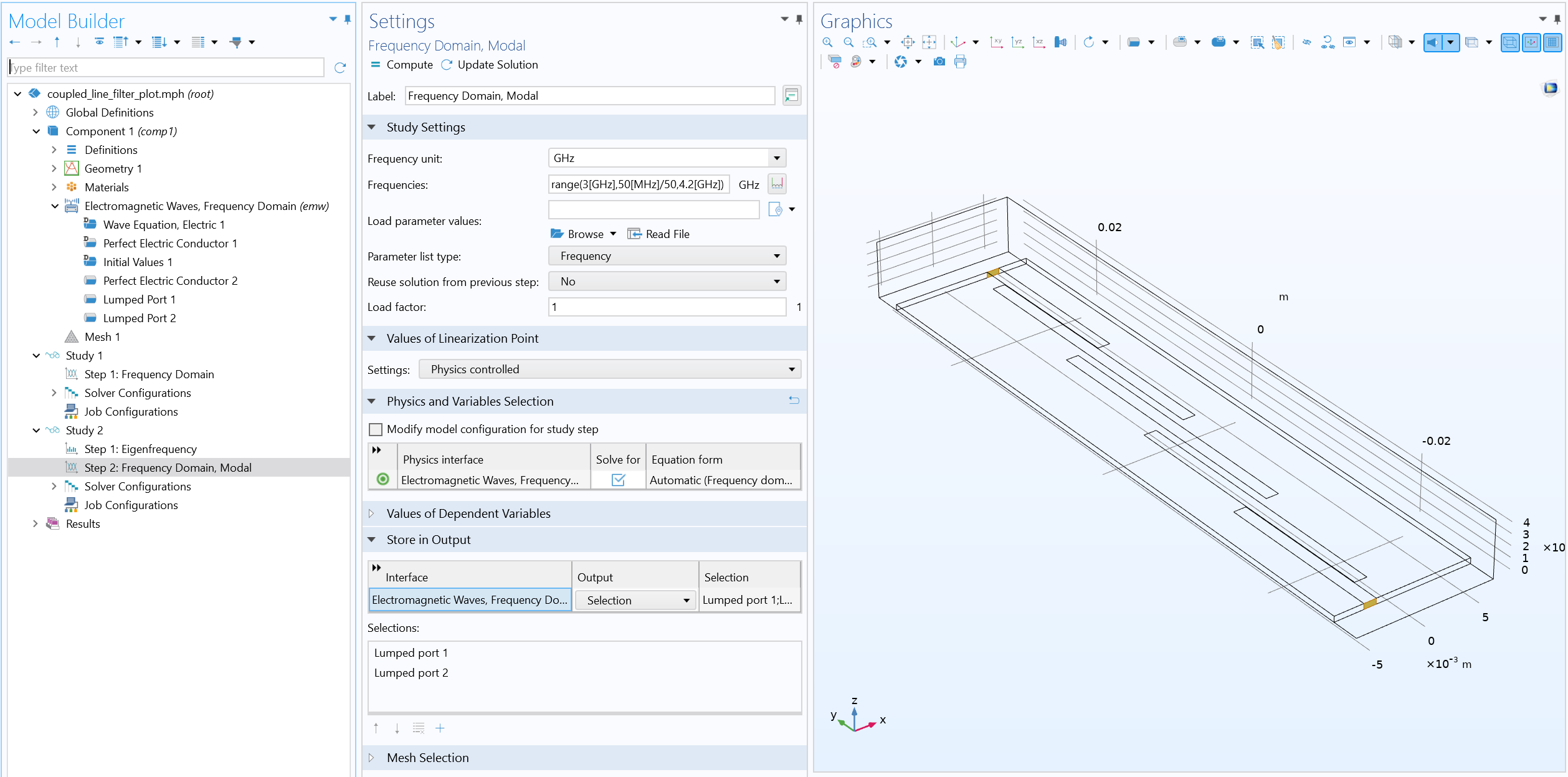 The Store in Output section of the Frequency Domain, Modal study step with two Lumped Port selections chosen. You can check the location of these selections in the Graphics window.
Available Application Gallery Examples
The simulation methods presented in this blog post are powerful tools for enabling faster, more efficient modeling of passive RF and microwave devices. Check out the following Application Gallery examples, which can provide further guidance in how to utilize these techniques:
- AWE method
- FDM method
Keep in mind that the methods and studies demonstrated here are universal and available not only for RF modeling. For example, you can also benefit from these methods when performing acoustic, mechanical, MEMS, and wave optics calculations.
Next Steps
Learn about other specialized features available for your RF and microwave modeling:


Comments (0)