Structural Mechanics Module Updates
For users of the Structural Mechanics Module, COMSOL Multiphysics® version 5.3 brings a modeling technique called stress linearization, a bolt pretension study step, and a boundary condition for rigid body suppression. Browse all of the new features and functionality in the Structural Mechanics Module below.
Stress Linearization Evaluation
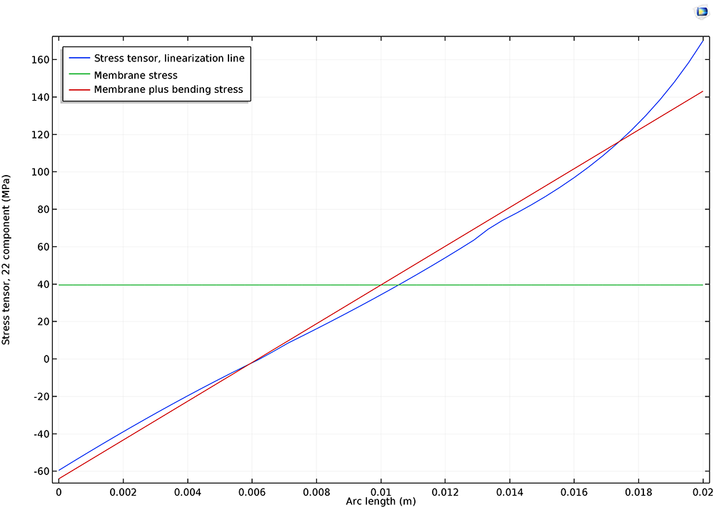
Stress linearization is a postprocessing technique where the stresses through a thin section in a solid model are represented by a constant membrane stress field and a linearly varying bending stress field. This type of evaluation is common when analyzing pressure vessels and is described in the ASME standard ASME Boiler & Pressure Vessel Code, Section III, Division 1, Subsection NB. Other application areas include computing reinforcement in concrete structures and some types of weld analyses.
The new Stress Linearization postprocessing node makes it possible to select the edges on which a stress linearization evaluation is to be performed. Membrane, bending, and peak stresses are reported and stress intensities are computed for each such stress classification line.
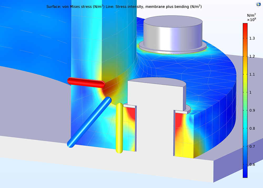 Three stress classification lines after being evaluated using the stress linearization technique. The lines (represented by tubes) on the face of the modeled flange show the maximum stress intensity with values as presented in the color bar. The surface plot depicts the von Mises stresses in the 3D object.
Application Library path for an example using the Stress Linearization postprocessing technique:
Structural_Mechanics_Module/Contact_and_Friction/tube_connection
Dedicated Study Step for Bolt Pretension
A new study type has been introduced and is intended for the first analysis step in models consisting of pretensioned bolts. The Bolt Pre-Tension study step directly solves for a bolt's predeformation, which is not accounted for in other study types. With this study step, you no longer need to manually set the activation status for the degrees of freedom associated with analyzing the bolts.

A design consisting of pretensioned bolts holding a bracket. The first Study node contains the new Bolt Pre-Tension study type in the model tree. The second one would then solve for a stationary analysis.
Application Library path for an example using the Bolt Pre-Tension study step:
Structural_Mechanics_Module/Tutorials/bracket_contact
Automatic Detection of Bolts in Symmetry Planes and Handling Their Modeling Conditions
Pretensioned bolts that have been cut by a symmetry plane are now automatically detected. Both the given pretension force and the computed bolt forces of the cut bolt are interpreted as if it were a full bolt, thus greatly simplifying the modeling workflow.
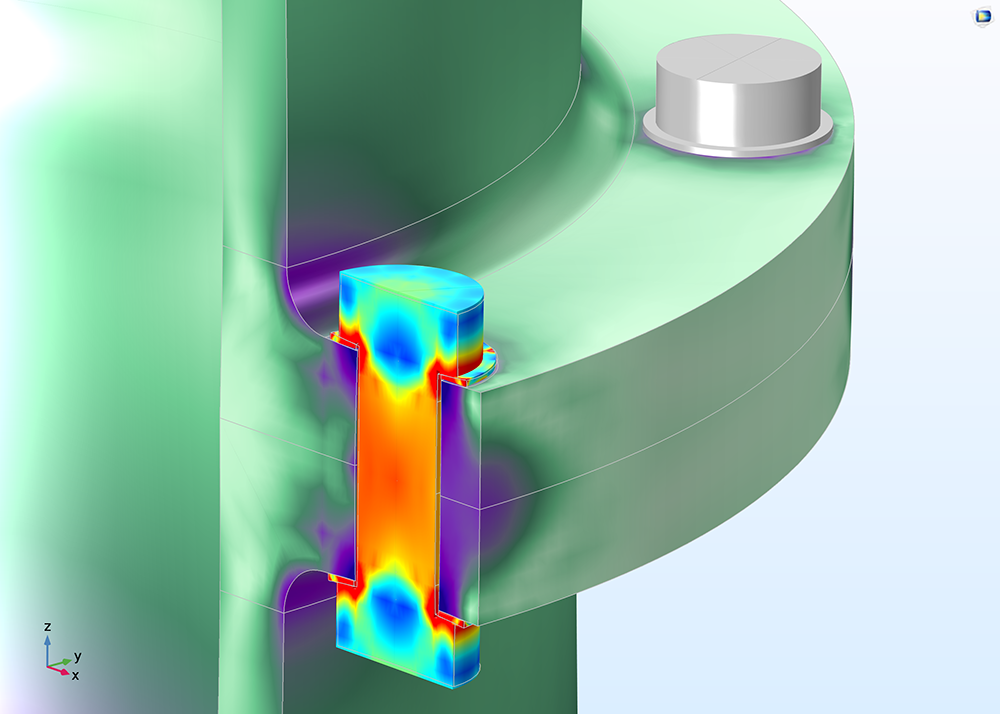 Stress plot of a pretensioned bolt that has been cut by a symmetry plane. The cut bolt is detected and treated as if it were a full bolt. This negates having to separately define bolts that have been cut by symmetry planes. All bolts in the model can be specified with the same conditions.
Application Library path for an example of automatically detecting bolts in symmetry planes:
Structural_Mechanics_Module/Contact_and_Friction/tube_connection
Automatic Suppression of Rigid Body Motion
In cases where loads are self-equilibrating, the actual locations of where the required constraints are placed are not relevant. Self-equilibrating models can be analyzed as long as the specifications of the constraints fulfill the following conditions: rigid body motions are not possible and no reaction forces are introduced. Now, the new Rigid Motion Suppression condition can be used for these types of analyses. This feature automatically applies a set of suitable constraints based on the geometry model and physics interfaces.
The Rigid Motion Suppression condition is available for the following physics interfaces:
- Solid Mechanics (3D, 2D, 2D axisymmetric)
- Shell (3D)
- Plate (2D)
- Membrane (3D, 2D)
- Beam (3D, 2D)
- Truss (3D, 2D)
- Multibody Dynamics (3D, 2D)

A heating circuit deforms due to thermal expansion in this example. Applying a Rigid Motion Suppression condition ensures that the model has sufficient constraints for a correct solution. The plot shows the von Mises stresses.
Application Library path for an example of rigid body motion suppression:
Structural_Mechanics_Module/Thermal-Structure_Interaction/heating_circuit
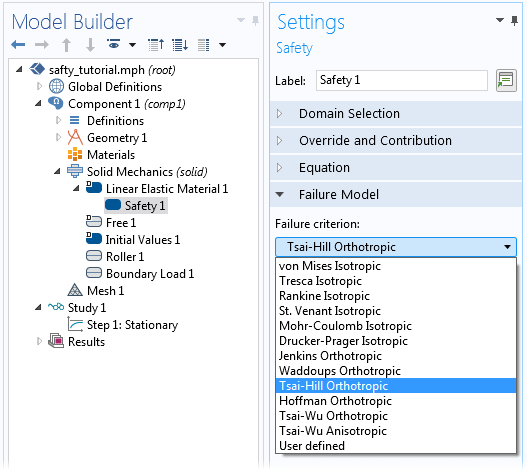
Computations of Safety Factors
The new Safety attribute to the Linear Elastic Material and Nonlinear Elastic Material nodes enables you to study the use of materials in the structure, particularly with respect to safety factors. The safety factor can be computed with respect to a large number of different isotropic, orthotropic, or anisotropic failure criteria, including user-defined expressions. When a Safety node is included, you can access postprocessing variables for the safety factor, margin of safety, and damage and failure indices.
Linear Buckling Analysis for the Beam Interface
You can now perform linearized buckling analyses in the Beam interface, facilitating the analysis of critical loads for various frame structures under compression. Additionally, models that use multiple and mixed structural mechanics interfaces can now also use this study or analysis type. This is because the analysis type is already available in other physics interfaces, such as the Solid Mechanics and Shell interfaces.
 The buckling shape of a space frame subjected to vertical loads.
Application Library path for an example of a buckling analysis for the Beam interface:
Structural_Mechanics_Module/Verification_Examples/space_frame_instability
New Data Set for Results from Shell Element Analyses
Many thin structures can be analyzed using shell elements and boundary meshes instead of 3D meshes in order to save computational resources. However, it can be difficult to visualize what is meant to be a 3D structure with results that differ between the top and bottom surfaces of the shell if you have to use shells in the postprocessing step. This becomes even harder when visualizing them effectively together with other 3D parts of your model, analyzed using 3D meshes.
With the new release of COMSOL Multiphysics®, you can plot results from a shell element analysis on two parallel surfaces and present them more effectively in a 3D visualization. By default, the surfaces are separated at a distance equivalent to the thickness used in the shell element analysis. Yet, you can manually modify this separation to improve visualization of very thin objects. All of this is achieved with the new Shell data set under the Results node.
Stress analysis of a bracket where certain parts of the geometry are analyzed using the Shell interface and other parts use the Solid Mechanics interface. When a Shell analysis is used to analyze the shell elements of this geometry, the default plot (shown here) presents the shells as two parallel surfaces separated by the thickness parameter of the shells, with the top surface colored in blue-green, while the parts of the geometry are 3D in nature have been hidden.
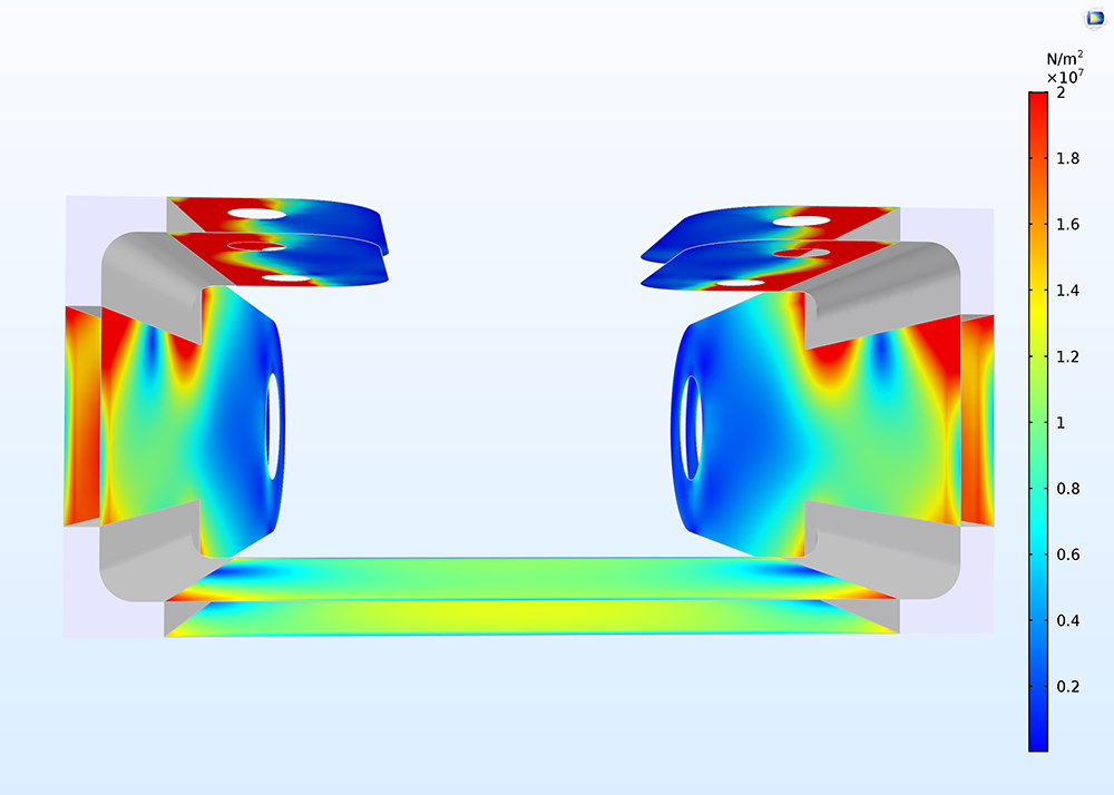
Stress analysis of a bracket where certain parts of the geometry are analyzed using the Shell interface and other parts use the Solid Mechanics interface. The plot here shows the stresses on both sides of the shells using the Shell data set (results on parts of the geometry modeled by solid elements are not shown).
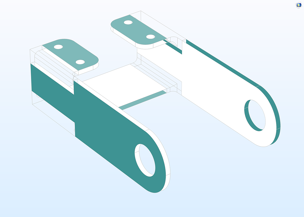
New Multiphysics Couplings Between Structural Mechanics Interfaces
Connecting different structural mechanics interfaces has been made significantly easier through the introduction of three new multiphysics couplings interfaces: Solid-Shell Connection, Solid-Beam Connection, and Shell-Beam Connection. As a result, the previous subnodes that could be added under the Solid Mechanics node — Beam Connection, Shell Connection, and Solid Connection — are now obsolete and have been removed. The Solid-Shell Connection and Solid-Beam Connection couplings are useful for connecting domains from either the Solid Mechanics or Multibody Dynamics interfaces.
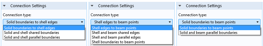
The available connection settings for the (from left to right) Solid-Shell Connection, Shell-Beam Connection, and Solid-Beam Connection couplings.
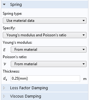
Elastic Layers Described by Material Data
You can now prescribe the elastic properties of a spring foundation or a thin elastic layer with material data such as Young's modulus and Poisson's ratio together with a given thickness of the layer. This simplifies, for example, the modeling of adhesive layers with known material properties. When using the material data and thickness as input, the strains in the elastic layer are also available as results.
Mode Analysis in Solid Mechanics
A new mode analysis study type has been added to the Solid Mechanics interfaces in 2D. Mode analysis is used to study mode shapes and wave numbers for waves traveling in the out-of-plane direction. Applications include general acoustic-structure interaction and nondestructive evaluation on cross sections. The Solid Mechanics interface in 2D axial symmetry has a new option for Circumferential mode extension and can be used with an Eigenfrequency study for computing circumferential mode shapes and mode numbers.
Note: The model in the example also requires the Acoustics Module.
 Propagation modes in the chamber of a muffler with thin elastic walls. Acoustic pressure and structural deformations are shown.
Application Library path for an example of the new mode analysis study type:
Acoustics_Module/Automotive/eigenmodes_in_muffler_elastic
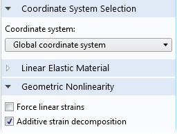
New Framework for Inelastic Strains in Geometrically Nonlinear Analyses
A new framework and more rigorous handling of decomposition into elastic and inelastic deformations has been implemented for cases of geometric nonlinearity. Previous versions of the COMSOL® software used an additive decomposition approach, with a few exceptions such as for large-strain plasticity analyses, which use a multiplicative decomposition approach.
Multiplicative decomposition is now also available for:
- Thermal Expansion
- Hygroscopic Swelling
- Initial Strain
- External Strain
- Viscoplasticity
- Creep
Multiplicative decomposition of deformation gradients is now the default option for all inelastic contributions in studies where geometric nonlinearity is active. The main advantage is that it is possible to handle several large inelastic strain contributions in a material. Furthermore, linearization will be more consistent as, for example, it is now possible to accurately predict the shift in eigenfrequencies caused by pure thermal expansion. If you want to switch to the behavior of previous versions of the COMSOL Multiphysics® software, the new Additive strain decomposition check box can be selected in the Settings window for the respective material models.
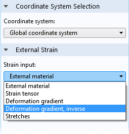
As part of this improvement, the External Strain attribute under the Linear Elastic Material and Nonlinear Elastic Material nodes has been expanded with several new options. These options allow for supplying inelastic strains in several forms and you can also transfer inelastic strains from other physics interfaces to this attribute. Additionally, an External Strain attribute with similar properties has been added to the Hyperelastic Material.
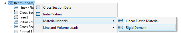
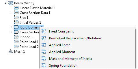
Rigid Domain in Shell and Beam Interfaces
The Rigid Domain material model is accessible from the Shell and Beam interfaces. This is an efficient modeling technique for parts that are significantly stiffer than their surrounding parts, since it only requires the degrees of freedom of a rigid body for an entire set of boundaries (Shell) or edges (Beam). Just as for the corresponding material model in the Solid Mechanics and Multibody Dynamics interfaces, you can apply loads, springs, and inertia at arbitrary locations on the rigid body.
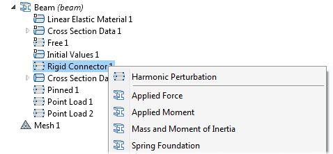
Rigid Connector in the Beam Interface
The Rigid Connector feature is now available for use in the Beam interface. A set of nodes can be selected to form a rigid region and be used, for example, to avoid overestimating the flexibility at beam connections. It can also be a means of applying off-center loads, springs, or extra inertia contributions.
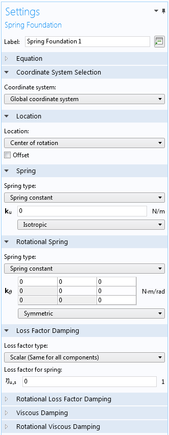
Spring Boundary Conditions for Rigid Domain and Rigid Connector
The Rigid Connector and Rigid Domain features in all physics interfaces have been augmented with a spring boundary condition called Spring Foundation. It has the following properties:
- The spring can be attached at an arbitrary position
- Both translational and rotational springs are available
- The spring can have loss factor damping
- The spring can act in parallel with viscous damping (for both translation and rotation)
Energy Quantity Variables for Modeling Contact
New variables containing energy quantities are available when modeling contact. You can now obtain the energy dissipated by friction as well as the elastic energy stored in the contact penalty factors. This is useful for checking energy balances as well as a posteriori checks on selected penalty factors.
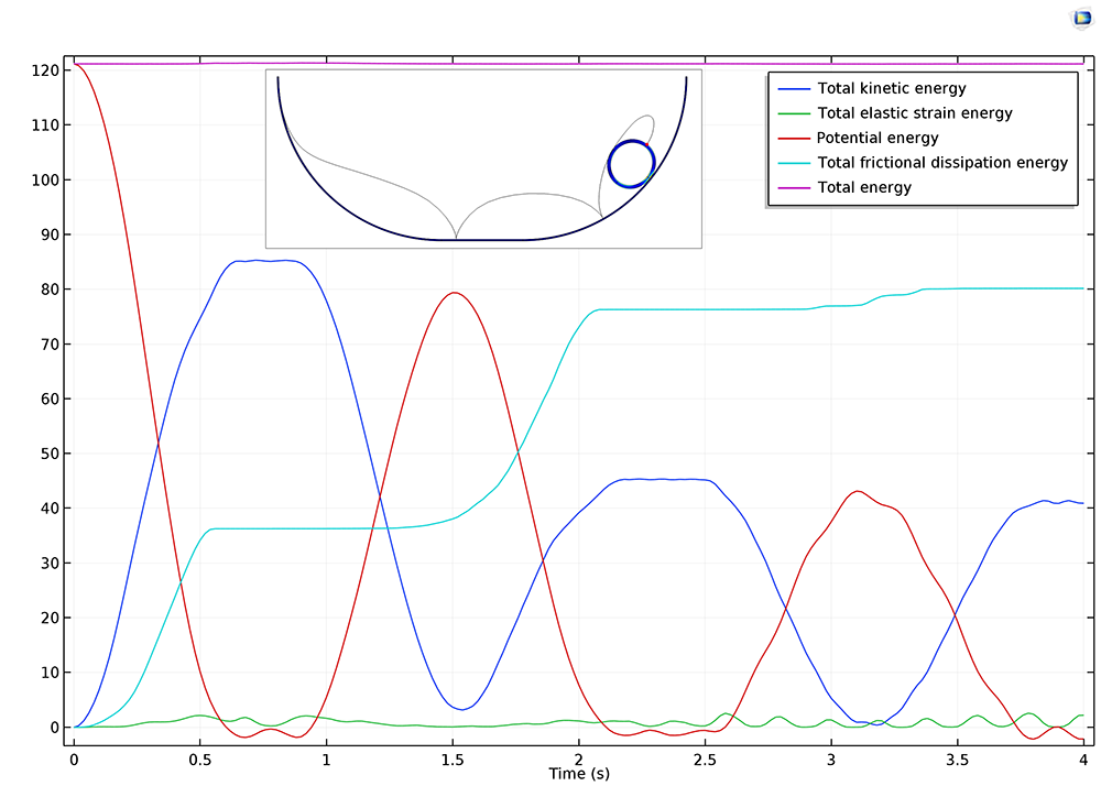 Energy balance for a cylinder rolling and sliding inside a channel due to gravity.
Application Gallery link for an example containing new variables for energy quantities when modeling contact:
Transient Rolling Contact
Frequency-Domain Analysis with Contact
You can study the frequency response of a structure where a contact state has been computed in a previous study. As an example, you can perform frequency-domain analyses of bolted structures and study the influence of contact states on the dynamic properties.
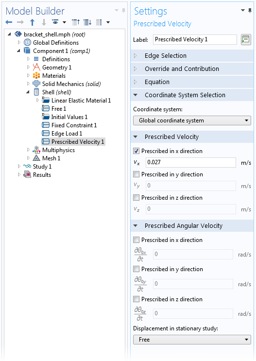
Harmonic Perturbation for Prescribed Velocity and Acceleration
In the Shell, Plate, and Beam interfaces, you can provide values for harmonic perturbation for the Prescribed Velocity and Prescribed Acceleration nodes.
Enhancements to Including Physics Symbols
You now have much better control over the display of physics symbols on geometries visualized in the Graphics window. These can be switched on or off, both within the respective physics interface Settings window and the settings for individual features under a physics node.
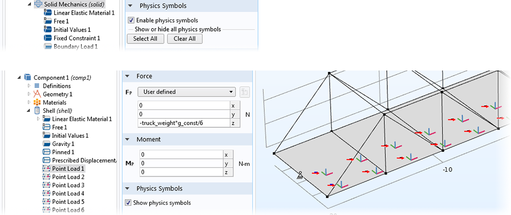
Switching between showing and not showing physics symbols in your model setup in the Graphics window. You can select the Enable physics symbols in the main node's (e.g., Solid Mechanics) Settings window (top) as well as in a single feature's (e.g., Point Load) Settings window (bottom).
Enhancements to Including External Material Functionalities
Several enhancements have been made with regards to the power and usability of material models created with user-defined C code:
- Inelastic strain contributions for nonlinear elastic and hyperelastic materials can now be implemented
- Two new interfaces to the C code that take several more quantities as input, including deformation gradients
- Now possible to include serendipity shape functions
- Small strain formulation has been added
- You can start by making a special initialization call to the user function
- You can make a cleanup call to the user function (e.g., closing files)
- The state variables can be named individually
- Time is available as an input argument
New Tutorial Model: Transient Rolling Contact
The Transient Rolling Contact example shows the concept of how to handle a transient contact problem with stick-slip friction transition. A soft hollow pipe subjected to gravity load is released at the top of a half-pipe. Its motion varies between sliding and rolling, depending on its position in the half-pipe and its velocity. The cross section of the pipe changes its oval shape due to contact and inertial forces. An energy balance validates the accuracy of the solution.
A soft pipe is dropped from the top region of a half-pipe and its motion and shape of the pipe's cross section is subject to gravitational and contact forces. Shown are the stresses in the pipe at a point in time as well as the trajectory of a point on the pipe as its motion varies between sliding and rolling.
Application Gallery link:
Structural_Mechanics_Module/Contact_and_Friction/transient_rolling_contact
New Tutorial: Noise Radiation by a Compound Gear Train
Predicting the noise radiation from a dynamic system gives designers insight into the behavior of moving mechanisms early in the design process. For example, consider a gearbox in which the change in the gear mesh stiffness causes vibrations. These vibrations are transmitted to the gearbox housing through shafts and joints. The vibrating housing further transmits energy to the surrounding fluid, resulting in acoustic wave radiation.
This tutorial model simulates the noise radiation from the housing of a gear train. First, a multibody dynamics analysis is performed in the time domain to compute the housing vibrations at the specified driver shaft speed. Then, an acoustic analysis is performed at a selected frequency to compute the sound pressure levels in the near, far, and exterior fields using the housing's normal acceleration as a noise source.
Note: This model also requires the Multibody Dynamics Module and the Acoustics Module.
Normal acceleration on the surrounding box of the moving gear train. In the model, the radiated acoustic pressure is also calculated.
Application Library path:
Acoustics_Module/Vibrations_and_FSI/gear_train_noise