In version 6.3 of the COMSOL Multiphysics® software, a new Concentrated Electrolyte Transport interface was introduced. This interface enables the modeling of electrolytes consisting of an arbitrary number of electrolyte species (anions, cations, and neutral solvents) at any concentration level. This blog post serves as an introduction to the new interface.
Background on Interfaces
In COMSOL Multiphysics®, there are various physics interfaces available for modeling ion concentration distributions in electrochemical cells. The Tertiary Current Distribution, Nernst–Planck interface (available in the Battery Design Module, the Fuel Cell & Electrolyzer Module, the Corrosion Module, the Electrodeposition Module, and the Electrochemistry Module), can define ion transport using various flavors of the Nernst–Planck equations. Common for all of these formulations is the usage of a dilute approach where the flux of each modeled species only relates to its own gradient in electrochemical potential, and where the composition of an assumed common bulk does not change as a result of the electrochemical reactions in the cell.
The Nernst–Planck flux definition is a suitable choice when there is a common neutral solvent species present in the solution at a high concentration in relation to all other species, limiting the impact of nonsolvent binary interactions. Another case where a Nernst–Planck-based approach can be used is to investigate the transport of a trace ion when there is a supporting electrolyte present. (A supporting electrolyte means that there is a large amount of additional ions present in the electrolyte, whose concentration can be considered constant.)
To handle transport in electrolytes where a solvent, or bulk supporting electrolyte, of constant concentration cannot be assumed, one has to switch from the Nernst–Planck approach to concentrated solution theory. Simply put, concentration solution theory means that we include concentration changes of all major species, including solvents that impact the current distribution in the cell. Concentrated formulations for electrolytes composed of three species, one cation, one anion, and one neutral solvent, are built into the Lithium-Ion Battery interface (available in the Battery Design Module).
There are some scenarios where the Tertiary Current Distribution, Nernst–Planck and Lithium-Ion Battery interfaces are not the best options for accurately describing ion transport. In those scenarios, the Concentrated Electrolyte Transport interface is ideal. A typical use case for this interface is demonstrated in the Molten Carbonate Transport tutorial, which is included in the Application Libraries of the Battery Design Module, Fuel Cell & Electrolyzer Module, Corrosion Module, Electrodeposition Module, and Electrochemistry Module. The model defines a salt melt consisting of \mathrm{Li}^+, \mathrm{K}^+, and \mathrm{CO}_3^{2-} that acts as the active electrolyte in a molten carbonate fuel cell with an initial molar proportion of the ions \mathrm{Li}_{0.38}\mathrm{K}_{0.68}(\mathrm{CO}_3)_\mathrm{0.5}. In this salt melt there is no neutral solvent present.
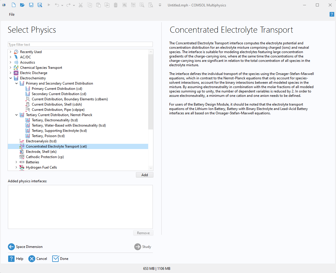 Selecting the Concentrated Electrolyte Transport interface in the Model Wizard.
Other examples where the Concentrated Electrolyte Transport interface could be applicable are when working with ionic liquids or battery electrolytes featuring multiple neutral solvents.
Concentrated solution theory formulations for a multitude of applications have been presented in literature over the years, most of which were pioneered by Newman and his colleagues (Ref. 1). The generalized formulation used in the Concentrated Electrolyte Transport interface is based on the works of Van-Brunt, Farrell, and Monroe (Ref. 2).
Onsager–Stefan–Maxwell Equations vs. Nernst–Planck Equations
The Concentrated Electrolyte Transport interface deploys an Onsager–Stefan–Maxwell approach for electrolyte transport. (Note: The transport equations used for gas phase transport in the Hydrogen Fuel Cell and Water Electrolyzer interfaces, and in the Transport of Concentrated Species interface, are derived following similar principles.)
The underlying idea of the Onsager–Stefan–Maxwell formalism (also referred to as Maxwell–Stefan in literature) is to define a force balance equation for every species transported in the electrolyte, which relates the gradient in the electrochemical potential \mu_i of each species to a sum of friction forces that occurs due to binary interactions with all other species. These friction forces depend on the relative transport velocities, \mathbf{v}_i, and concentrations, c_i, of the species being involved in the interactions.
For general cases, the Onsager–Stefan–Maxwell force balance for any species in the electrolyte reads as
Here, c_T is the total concentration of all electrolyte species, and D_{i,j} denotes the binary diffusivities of all species pairs in the solution. The left-hand side above represents the driving force for transport and relates to the gradient of the Gibb’s free energy of the electrolyte species of index i. The right-hand side represents the friction forces, expressed as a sum over all interactions between species i and all other species.
The above equation is formulated for all n species of the solution, which results in n-1 independent force balances. The number of required transport parameters is n(n-1)/2.
For the \mathrm{K}^+ ion in our molten carbonate salt melt example, the force balance becomes
where c_T=c_\textrm{K}+c_\textrm{Li}+c_\textrm{CO3}.
Introducing the definition
for the molar flux \mathbf{N}_i for the species, we can rewrite the above expression as
Similar force balances are also formulated for \mathrm{Li}^+ and \mathrm{CO}_3^{2-}.
Since all three ions are present in the electrolyte at comparable concentrations, it is hard to formulate a Nernst–Planck model for the electrolyte transport. In order to see how the fluxes as computed by the Onsager–Stefan–Maxwell approach relate to the ion flux as defined by the Nernst–Planck equations, we need to add an additional (fictitious) neutral solvent species S to the electrolyte.
The force balance for \mathrm{K}^+ now reads as
If the solvent is in excess, we may assume that c_T \approx c_\textrm{S} and that all terms containing c_\textrm{K}/c_\textrm{T}, c_\textrm{Li}/c_\textrm{T}, and c_\textrm{CO3}/c_\textrm{T} may be neglected in the above expression. This results in a simplified force balance:
Let’s now turn our attention to the electrochemical potential on the left, which is defined as
where \lambda_\textrm{K} is the thermodynamic factor and x_\mathrm{K} is the molar fraction of \mathrm{K}^+. z_\textrm{K}=1 is the \mathrm{K}^+ ion charge and \Phi is the electrolyte (solution) phase potential.
Assuming ideal conditions (we will discuss nonidealities later on), we may replace the thermodynamic factor and molar fraction with the concentration when computing the gradient of the electrochemical potential. Inserting this into the simplified force balance results in
which may be rearranged to
which is the flux definition used for the individual ions in the Tertiary Current Distribution, Nernst–Planck interface (when using the Nernst–Einstein relation to define the mobility).
To sum up what we’ve seen with these equations: The Onsager–Stefan–Maxwell ion flux definition for an ion at infinite dilution is asymptotically equal to the Nernst–Planck flux.
Other Sets of Transport Parameters
The Concentrated Electrolyte Transport interface makes use of binary diffusivities to form the set of needed n(n-1)/2 transport parameters. Using binary diffusivities is the most generic way to formulate transport parameters. However, there are other ways of formulating the transport parameters in the concentrated solution theory.
For our salt melt example, it would be possible to transform the transport equations into a set containing:
- The electrolyte conductivity
- A salt diffusivity for one of the neutral salts
- A migration coefficient
The conductivity then relates to the binary diffusivities as
}{
c_\textrm{K}D_\textrm{Li,CO3}+ c_\textrm{Li}D_\textrm{K,CO3}+ c_\textrm{CO3}D_\textrm{Li,K}
}.
Another example is the Lithium-Ion Battery interface, which uses the three parameters, conductivity, the salt diffusivity, and the transport number, as a basis. Conversion formulas exist in literature (Ref. 2) to convert between these different ways of defining transport parameters.
It should be noted that regardless of the formulation, the transport parameters are generally composition-dependent.
Electrolyte Species, Electroneutrality, Electrolyte Components, and Molar Constraint
As already touched on, an electrolyte consists of one or several cations (positively charged ions), one or several anions (negatively charged ions) and, optionally, additional neutral solvents. Denoting the total number of different electrolyte species as n, this results in n+1 dependent variables (unknowns) to solve for: n concentrations and one solution potential. However, by the use of two algebraic constraints, the number of dependent variables may be reduced.
Firstly, due to the large energies required to separate charges at distances relevant to electrolyte transport modeling, electroneutrality is commonly assumed in electrochemical cell modeling, and so is the case for the Concentrated Electrolyte Transport interface. Electroneutrality means that at any location in space, we define the net space charge (that is, the sum of all species concentrations times their individual charges) to equal zero:
The electroneutrality condition provides an algebraic equation that can be used to remove one dependent variable from the equation system. (The same electroneutrality condition is also used in the Tertiary Current Distribution, Nernst–Planck interface.)
When setting up the transport equation system for a concentrated electrolyte, it turns out that, as a result of the electroneutrality condition, it is convenient to make use of a set of electroneutral electrolyte components to use as a basis to define the dependent variables, instead of the individual charged ions. Here, we define an electroneutral electrolyte component either as a neutral binary salt (anion + cation) or a neutral solvent. In the Concentrated Electrolyte Transport interface, a set of electroneutral components is created automatically based on the number of anion and cations and their individual charges.
It should be noted that the space of the possible electrolyte component basis is often not unique and that the neutral salts defined in the basis need not have any connection to the actual salts used in practice in the lab for producing the electrolyte mix — they are pure mathematical entities that facilitate handling the electrolyte transport system and the definition of electroneutral initial and inlet boundary conditions.
Secondly, to further reduce the number of dependent variables in the system, we make use of a molar fraction constraint where we define the molar fractions of all species to sum up to unity. The molar fraction constraint is:
where x_i = c_i/c_T.
As a result of two algebraic equations, the electroneutrality condition and the molar fraction constraint, the number of dependent variables we need to solve for in a system consisting of n electrolyte species gets reduced from n+1 to n-1.
Internally, the Concentrated Electrolyte Transport interface makes use of a number of matrix operations in order to convert between variables expressed in the electrolyte component basis and variable expressions based on the individual species. As a user, however, only limited considerations need to be made with regard to the electrolyte component versus the species basis. User input for flux and source expressions, which are not constrained to be electroneutral, are typically expressed in terms of the individual electrolyte species, whereas user input specifying the electrolyte composition such as in the Initial Values and Inflow nodes are specified using the electrolyte component basis in order to ensure electroneutrality. Many results evaluation variables are defined in both bases.
We’ll now summarize the concepts covered in this section by looking at the Settings window of the top node of the Concentrated Electrolyte Transport interface for our molten carbonate tutorial example.
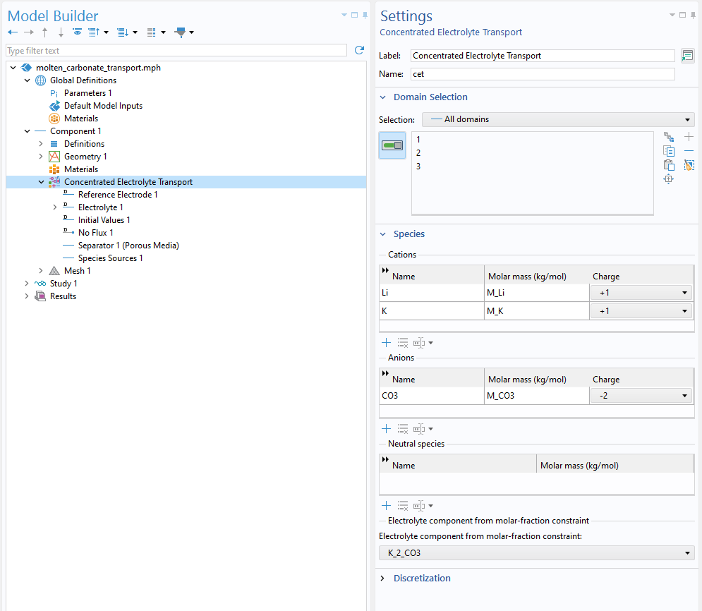 The Settings window for the Concentrated Electrolyte Transport interface.
Here, we specify the names of the two cations, \mathrm{Li}^+ and \mathrm{K}^+, and the anion \mathrm{CO}_3^{2-}, along with their corresponding charges. The list of neutral solvents is kept empty. From this set of ions, the Concentrated Electrolyte Transport interface automatically generates the two neutral salts, \textrm{Li}_2\textrm{CO}_3 and \textrm{K}_2\textrm{CO}_3, as electrolyte components. The Electrolyte component from molar-fraction constraint setting enables us to choose which corresponding dependent variable to solve for. (What electroneutral components we choose to solve for as dependent variables may impact the numerical stability when solving the equation system, but it usually does not matter that much). This setting will also affect how nonideal thermodynamic factors are defined, as explained below.
Also note that the molar masses of all species need to be provided in this Settings window. The molar masses are used in various places in the interface in order to compute variables such as induced convective velocities, mass fractions, and the electrolyte density from average molar volumes.
The Reference Electrode
Unique for the Concentrated Electrolyte Transport interface, in comparison with the other Electrochemistry interfaces in COMSOL Multiphysics®, is the Reference Electrode domain node, which is added by default and is active on all domains. On this node, the stoichiometric coefficients of a common reference electrode reaction are defined, which in turn are used when defining the electrolyte phase potential variable.
Why do we need to define this common reference electrode? The need arises if we cannot assume ideal activities of the electrolyte species. A deepened discussion regarding how to consistently define the electrolyte phase potential is beyond the scope of this blog post (I’ll refer the interested reader to the references below), but the reason for why it is practical to define a common reference electrode stems from electroneutrality, and the practical impossibilities that relate to measuring the electrochemical activity of a single ion only. Simply put: One cannot vary the concentration of a single ion in an electrolyte without at the same time altering the concentration of another ion in order to maintain electroneutrality. For diluted electrolytes, the use of ideal activities may be motivated, or one could use Debye–Hückel theory, or related expressions, to define ion activities. However, these activity expressions are only valid for concentrations up to 0.1 M, so for a concentrated electrolyte we usually have no practical way of assessing the activity of individual ions.
By the introduction of the reference electrode, some of the difficulties are circumvented when it comes to defining a consistent electrolyte potential for nonideal concentrated electrolytes.
For our molten carbonate fuel cell example, the following reaction occurs at the cathode:
whereas on the anode we have
Inspecting the two reactions above, we see that the stoichiometry of the \mathrm{CO}_3^{2-}, which is the only electrolyte species, is the same (= 1) in both reactions. By convention, the species becoming oxidized in a reduction reaction gets a positive sign. Since we have a common ion reacting on both electrodes, a suitable choice of reference electrode stoichiometry for this model is to only include \mathrm{CO}_3^{2-} and set the coefficients of all other ions to 0. (Similarly, in the Lithium-Ion Battery interface, the electrolyte phase potential is defined with reference to an electrode with a unit lithium-ion stoichiometry.)
The corresponding Settings window looks like this in the example model:
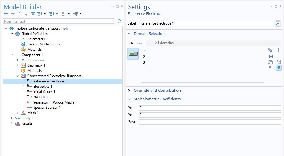 The Settings window for Reference Electrode showing the stoichiometric coefficients for the molten carbonate fuel cell example.
By this definition of the reference electrode reaction, any concentration changes of \mathrm{CO}_3^{2-} are inherently built into the electrolyte phase potential definition, and the definition of this electrolyte potential will also be consistent with any nonideal thermodynamic factors defined on the Electrolyte node (see next section). This means that when we later on define overpotential variables for kinetics for usage in kinetic expressions, no additional Nernstian concentration corrections need to be made.
Electrochemistry-Induced Convection
Convection may be induced electrochemically in the cells. This may occur both as a direct result of inserting or extracting ions at an electrode–electrolyte interface, or indirectly as a consequence of density changes when the electrolyte composition varies.
The Electrolyte node contains settings for setting both the velocity and the density of the electrolyte.
For a transient simulation, the velocity would typically be computed by a Fluid Flow interface in COMSOL Multiphysics®, where the composition-dependent density computed by the Concentrated Electrolyte Transport interface would be used as input in the continuity equation. The Concentrated Electrolyte Transport interface also computes a number of additional variables, such as net mass sources and boundary velocities that can be accessed from within a Fluid Flow interface.
The Reference-electrode-stoichiometry based velocity setting can be used as a simplification to define a velocity without the need for a separate Fluid Flow interface. The setting assumes that the total mass flux stems only from reactions with the same stoichiometry as defined in the Reference Electrode node. In many cases, such as in our stationary example model, this assumption is legit.
In our example model, the Settings window for the Electrolyte node looks as follows. Here, we are using a user-defined expression for the Density, which depends on the ion concentrations as defined under Definitions higher up in the model tree.
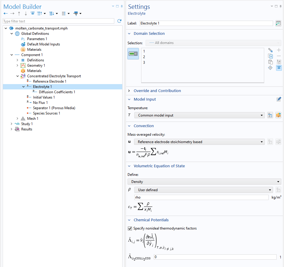 The Settings window for the Electrolyte node, where the velocity is defined with the Reference-electrode-stoichiometry based velocity setting and the density is user defined.
Chemical Potentials and Nonideal Activities
The Chemical Potentials section of the Electrolyte node allows for defining nonideal thermodynamic factors. (In our example, we are using ideal activities with the factor set to 1 for all individual species.)
To consistently define the chemical potentials of a concentrated electrolyte, two considerations need to be made: 1) We cannot change the fraction of a single electrolyte component without also changing the fraction of another component. 2) Although the fraction of an electrolyte component is kept constant, the chemical activity of that component may be impacted when the fractions of other components change.
As a result of these two considerations, plus some additional thermodynamic relations (see Ref. 2), (n-2)(n-1)/2 component thermodynamic factors are required to define the nonideal chemical activities of an electrolyte consisting of n species.
The nomenclature for defining the thermodynamic factors, and its index notation in the user interface, is a bit complex and merits some attention on its own. The generic user-interface formula reads as
The tilde (\tilde{}) notation here means we are referring to electrolyte components rather than individual species, so that \tilde{y}_j and \tilde{\lambda}_j refer to the electrolyte component fraction and electrolyte component activity, respectively. The stoichiometric factor \tilde{\nu}_i equals 1 for single-species components (neutral species) and the total number of ions in the formula unit for salts.
The lower-right subfix refers to properties kept constant while carrying out the derivative.
The formula should hence be interpreted as the activity change of an electrolyte component i when changing the fraction of component j, which is accomplished by simultaneously varying the electrolyte component k (but only that one). In the Concentrated Electrolyte Transport interface, the electrolyte component k will be the same one as set to be taken from the molar fraction constraint on the interface top node.
For our example containing the two electrolyte components \textrm{Li}_2\textrm{CO}_3 and \textrm{K}_2\textrm{CO}_3 only, we are left with a single thermodynamic factor, (3-2)(3-1)/2=1, whose formula gets rewritten as
Laying the Foundation for More Advanced Modeling
We’ll now finalize this blog post by looking at a result plot from the molten carbonate transport interface.
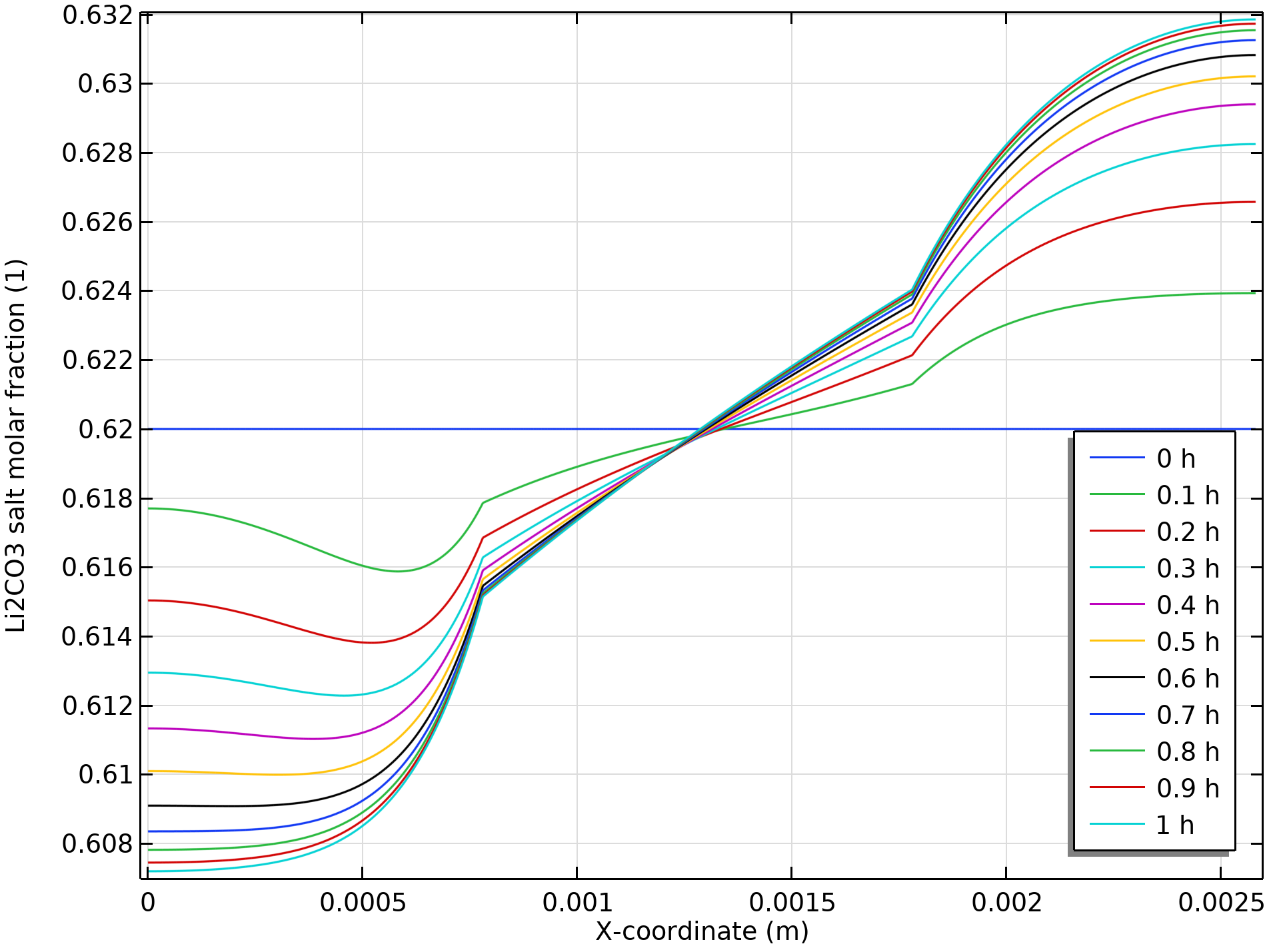 The results plot. The blue line at 0.62 is the initial value when the simulation starts. As time progresses, a salt separation gradient is built up in the cell.
The figure shows the fraction of \mathrm{Li}^+ ions in relation to the total amount of cations (\mathrm{Li}^+ and \mathrm{K}^+) in the molten carbonate fuel cell at various times. Over time we see a slight separation of the two cations in the cell, although neither of the two ions participate in the electrode reactions. The induced concentrations gradients may not seem dramatic, but it should be noted that the salt composition is closely related to how the electrolyte wets the porous matrices of the two electrodes. These small composition changes may result in secondary effects by affecting the electrolyte volume fraction in the electrodes, something that could be included in an extended model by introducing capillary pressure data and two-phase transport. No other physics interface in COMSOL Multiphysics® is capable of predicting the ion separation presented here.
Next Step
In this blog post, we highlighted the capabilities of the new Concentrated Electrolyte Transport interface using the Molten Carbonate Transport tutorial model. If you want to explore this interface and tutorial model yourself, click the button below.
References
- J. Newman et al., Electrochemical Systems, John-Wiley & Sons.
- A. Van-Brunt, P. Farrell, and C. Monroe, “Structural electroneutrality in Onsager–Stefan–Maxwell transport with charged species,” Electrochimical Acta, vol. 441, article 141769, 2023.


Comments (0)