
Composite materials are heterogeneous materials composed of at least two constituent materials. Among the different types of composite materials, layered composite materials are quite common and are widely used for aircraft, spacecraft, wind turbine, automobile, marine, buildings, and safety equipment use cases. The Composite Materials Module, an add-on to the COMSOL Multiphysics® software, includes built-in features and functionality specifically designed for studying layered composite structures. Fiber-reinforced polymers, particulate-reinforced polymers, laminated plates, and sandwich panels are a few common examples of layered composite materials.
Editor’s note: The original version of this post was written by Pawan Soami and published on December 6, 2018. It has since been updated to reflect new functionality.
Table of Contents
- What is a Composite Material?
- Micromechanics Analysis
- Macromechanics Analysis
- Laminate Theories and Physics Interfaces
- Material Models
- Results Evaluation Tools for Composite Material Modeling
- Multiphysics Analyses of a Composite Laminate
- Optimization of Composite Laminates
- Multiscale Analysis
What is a Composite Material?
Composite materials have specialized mechanical, thermal, electrical, and magnetic properties for specific applications, which is why they have many potential use cases in diverse areas. For instance, some industries are developing “smart” composite materials, which could have sensing, actuation, computation, communication, and other functionality. In structural engineering, composites are stronger and lighter than the conventional monolithic materials, which popularize their use. Before designing composite structures out of these materials, engineers must have a good understanding of their behavior.
Benefits and Challenges of Using Composite Materials
Composite material can be engineered to offer several advantages when compared with conventional materials, for example:
- High strength-to-weight ratio
- High impact resistance
- High resistance to fatigue and corrosion degradation
- Improved friction and wear properties
- Low thermal conductivity and low coefficient of thermal expansion
- High heat resistance
Since composite materials are a mixture of several materials, there are also some challenges involved when using these materials, including:
- Anisotropic material behavior
- Complex damage and failure modes
- High cost of raw materials and fabrication
- Difficulty in reuse and disposal
- Difficulty in joining different components
Industries that Use Composite Materials
Due to the abovementioned benefits, the use of composite materials is widespread in areas like:
- Aerospace engineering (e.g., wings, fuselages, and structural panels in satellites)
- Defense (e.g., tanks and submarines)
- Wind turbines (e.g., blades)
- Building and construction (e.g., doors, panels, frames, and bridges)
- Chemical engineering (e.g., pressure vessels, storage tanks, piping, and reactors)
- Automobiles and transportation (e.g., bicycle and automobile components)
- Marine and railway transportation (e.g., boat hulls and rail components)
- Consumer and sports goods (e.g., tennis rackets and golf club shafts)
- Electronics (e.g., distribution pillars and link boxes)
- Orthopedic aids
- Safety equipment
Types of Composite Materials and Their Classifications
There are several ways to classify composite materials, one of which is to categorize them based on constituent type, namely matrix and reinforcement. Based on the type of matrix material, composite materials can be classified into the following categories:
- Polymer matrix composites (PMC)
- Metal matrix composites (MMC)
- Ceramic matrix composites (CMC)
- Cement matrix composites (CeMC)
Based on the reinforcement types, composite materials can be classified into the following categories:
- Fiber composites
- Whisker composites
- Particulate composites
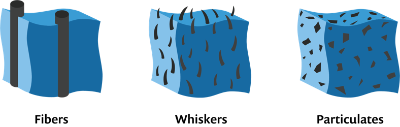
Examples of fiber, whisker, and particulate composites.
Fiber-Reinforced Polymers
Among other laminated composite materials, fiber-reinforced polymers (FRPs) are quite popular these days. These materials typically consist of a long fibrous part, which acts as the main load-carrying element, and a surrounding matrix, which supports the fiber and transfers the load. The fibers are arranged in a specified orientation in each layer (or lamina) of the material. A number of such laminae are stacked to form a laminated composite material that can be used to build a structural component. Fibers for industrial uses are, in general, made of carbon, glass, aramid, or boron. Based on the type of fiber material, the two most popular FRPs available and typically used in the industry are carbon-fiber-reinforced polymers (CFRP) and glass-fiber-reinforced polymers (GFRP), also known as fiberglass. Depending on the fiber orientations, the fiber composites can also be classified as unidirectional fiber composites or bidirectional fiber composites.
In this blog post, we will focus on unidirectional fiber-reinforced polymers, though it is possible to analyze any anisotropic laminated composite using the Composite Materials Module.
Types of Laminates
A composite laminate is defined as the stacking of two or more layers/plies/laminae with a uniform or varied fiber orientation with respect to a reference direction. The laminae can be made of the same material or different ones and can have individual thicknesses. The stacking sequence is essentially defined by the angle between the first principal material direction of each ply and the first axis of the laminate coordinate system.
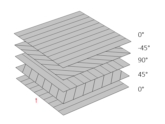
Stacking sequence (0/45/90/-45/0) of an antisymmetric balanced laminate.
Based on the stacking sequence, composite laminates can be classified into the following categories:
- Angle-ply laminate (e.g., 45/30/-45/-30)
- Cross-ply laminate (e.g., 0/90/0/90)
- Symmetric laminate (e.g., 45/30/30/45)
- Antisymmetric laminate (e.g., 45/30/-30/-45)
Analyzing a composite laminate can be rather challenging, as the geometric scale of fibers, plies, and laminates are quite different. This is why the analyses are often performed at different scales: at the microscale (micromechanics), the macroscale (macromechanics), or at both scales (multiscale analysis).
Micromechanics Analysis
A micromechanics analysis focuses on the composite materials at its constituent levels. It considers the constituent materials, the interface between them, and their internal arrangement. A micromechanical analysis is not limited to computing the homogenized material properties only, but is also useful for understanding the microlevel stresses, strains, nonlinearities, failures, damages, etc. Micromechanics-based homogenization techniques can be classified into two main types:
- Analytical methods (e.g., rule of mixtures)
- Numerical methods (e.g., finite element analysis using representative volume element (RVE) or repeating unit cell (RUC))
Under the Materials node in the Model Builder tree, the Multiphase Material and Effective Material nodes have several rules of mixtures for computing the effective properties analytically. The Effective Material node comes with the Composite Materials Module and has the following rules of mixtures:
- Volume average
- Mass average
- Harmonic volume average
- Harmonic mass average
- Power law
- Heaviside function
- Voigt–Reuss model
- Modified Voigt–Reuss model
- Chamis model
- Halpin–Tsai model
- Halpin–Tsai–Nielsen model
- Hashin–Rosen model
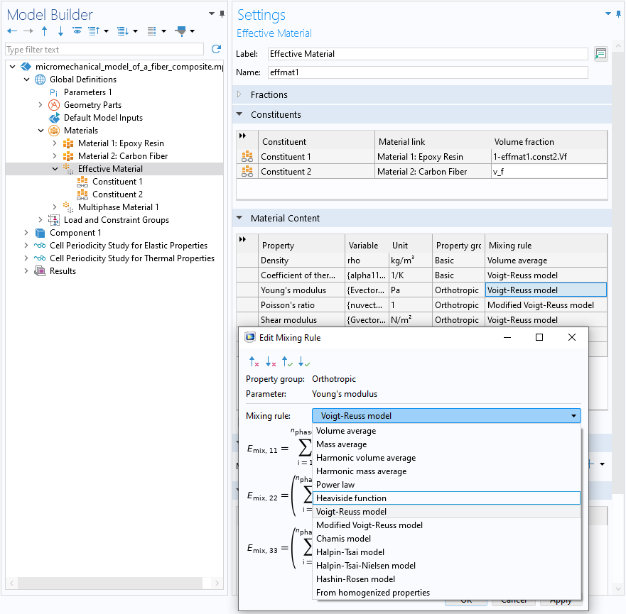
The Effective Material feature settings showing the Mixing Rule options.
To compute homogenized material properties numerically using the finite element method, we need either an RVE or RUC. For periodic materials, the RVE can be the same as the RUC, but for nonperiodic materials, the concept of RUC is not valid and thus the RVE material subvolume must be used.
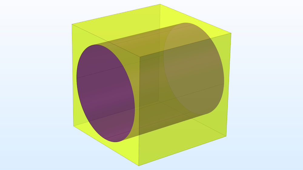
The unit cell of a fiber composite layer having a 60% fiber volume fraction.
In COMSOL Multiphysics®, micromechanics-based homogenization is performed using the Cell Periodicity node in the Solid Mechanics interface. It has two different boundary conditions, Periodic and Homogeneous. The Periodic boundary condition is applicable to the periodic materials and needs an RUC material subvolume. For nonperiodic materials, the Homogeneous boundary conditions can be applied with an RVE material subvolume. In this blog post, we focus on homogenized material properties of a unidirectional fiber composite, which is a periodic material.
The analysis starts with a geometry of a unit cell with a fiber and matrix. The material properties of the fiber and matrix need to be given. Then the action buttons in the Cell Periodicity node can be used to set up the required model nodes and study. The autocreated study computes the material data for a homogenized material.
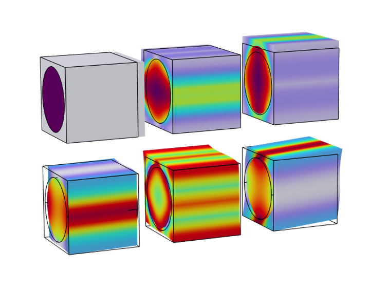
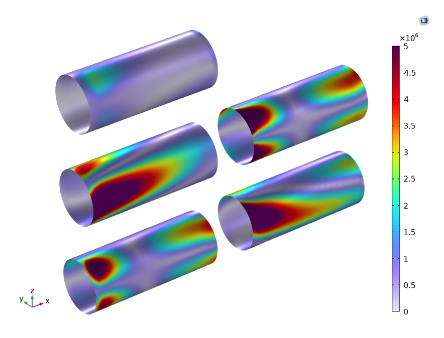
The von Mises stress distribution together with the deformation in a unit cell for six different load cases.
You can check out the Micromechanical Model of a Fiber Composite and Micromechanics and Stress Analysis of a Composite Cylinder examples to learn more.
Macromechanics Analysis
A macromechanical analysis determines the response of the composite structures based on the homogenized materials. The homogenized material properties of a lamina is obtained either from the micromechanics analysis or from experimental methods. The aim is to compute the response of a laminate at the global scale with various loading and boundary conditions. There are different steps in the macromechanical analysis, which are explained below.
Preprocessing Tools for Composite Material Modeling
To model a composite laminate, the following properties need to be specified:
- Number of layers
- Homogenized material properties of each layer
- Orientation of the principal material directions of laminate
- Thickness of each layer
- Stacking sequence
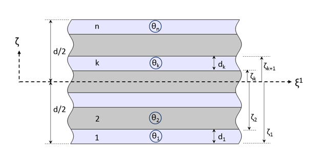
Cross section of a composite laminate showing the thickness and fiber orientation of each layer.
To define the laminate properties, a Layered Material node is used. In this node, the required number of layers can be added, and inputs can be either directly entered in the table or loaded from a text file. Once the inputs are specified, it is possible to preview the cross section as well as the stacking sequence of the laminate. The layered material containing the laminate definition, can be saved in the material library and loaded at a later point in time.
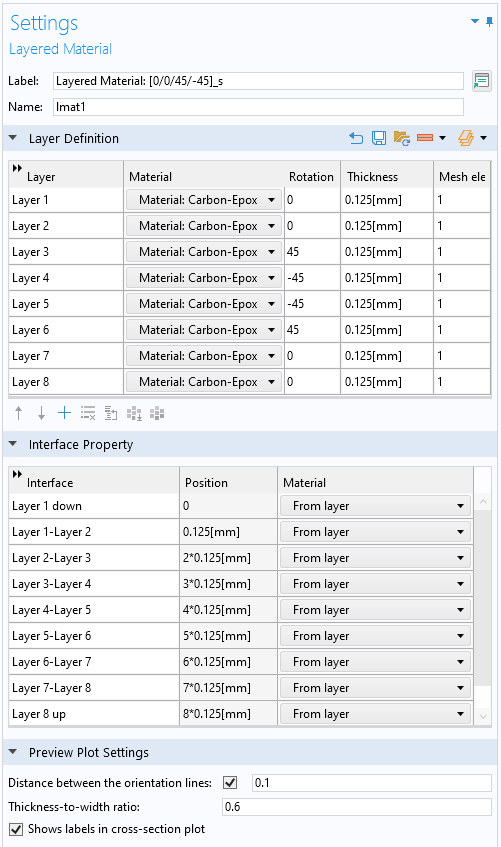
Example of a Layered Material node.
Once the laminate is defined using the Layered Material node, it can be attached to the geometric boundaries through the Layered Material Link or Layered Material Stack node. While doing so, the laminate coordinate system as well as the position of the geometric surface with respect to the laminate are also defined. The laminate coordinate system is further used to interpret the stacking sequence and create a layerwise local coordinate system. The Layered Material Link and Layered Material Stack nodes have further options to transform the layered material into symmetric, antisymmetric, or repeated laminates. They also include the option to model a spatially varying thickness. The Layered Material Stack node can be used for zone modeling, where the stacking sequence of the composite varies in different geometric selections.
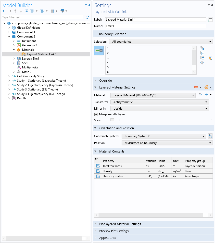
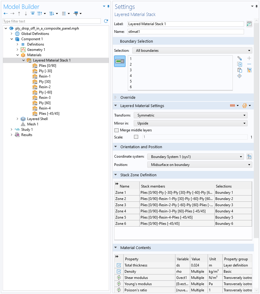
Examples of using the Layered Material Link and Layered Material Stack features.
Note that the Single Layer Material feature is a special version of Layered Material designed for single layer.
Laminate Theories and Physics Interfaces
Now that the laminate is defined and attached to geometric boundaries, let’s take a look at the laminate theories. The analysis of laminated composite shells is commonly based on one of three different theories:
- Equivalent single layer (ESL) theory
- Classical laminated plate theory (CLPT)
- First-order shear deformation laminated plate theory (FSDT)
- Higher-order shear deformation laminated plate theory
- Three-dimensional elasticity theory
- 3D elasticity theory
- Layerwise theory
- Multiple model methods
Equivalent Single Layer Theory (ESL-FSDT): Shell Interface
In ESL-FSDT, homogenized material properties of the entire laminate are computed and equations are solved only at the midplane. This theory has a shell-like formulation with degrees of freedom (DOFs) in the form of three displacements and three rotations on the meshed boundary. This theory is suitable for thin to moderately thick laminates and can be used for finding the global response as gross deflections, eigenfrequencies, critical buckling load, and in-plane stresses. Compared to the layerwise theory, ESL-FSDT is computationally inexpensive; however, it requires a shear correction factor for thicker laminates.
DOF nodes in ESL-FSDT.
In COMSOL Multiphysics®, the layered material features like Linear Elastic Material, Layered; Hyperelastic Material, Layered; and Piezoelectric Material, Layered in the Shell interface are based on ESL-FSDT theory. There is also a Linear Elastic Material, Layered feature in the Membrane interface based on the ESL theory, which can be used for modeling very thin composite films with negligible bending stiffness.
In the Stress and Modal Analysis of a Wind Turbine Composite Blade example, a wind turbine composite blade is modeled using the Shell interface. The aim of the analysis is to find the stress distribution in the skin and spar under gravity and centrifugal forces.
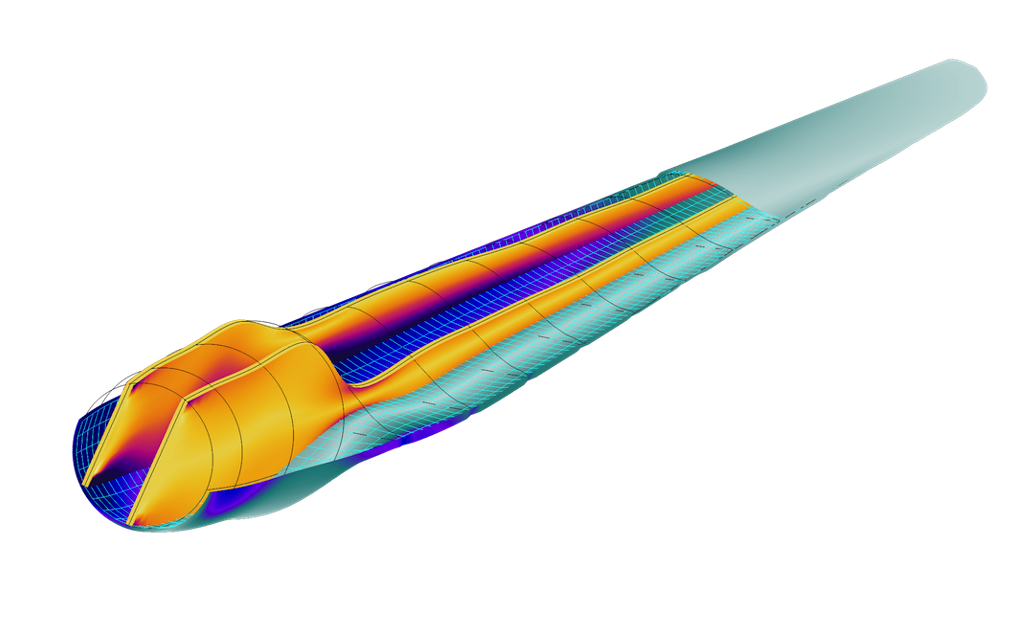
Example of a wind turbine composite blade. The von Mises stress distribution in the skin and spar of the blade is shown.
You can also check out the following examples to learn more:
Layerwise Theory: Layered Shell Interface
In this theory, equations are solved also in the thickness direction; hence, it can be used for very thick laminates, including delaminated regions. This theory has a solid-like formulation with DOFs in the form of three displacements distributed also in the thickness direction. This theory is suitable for moderately thin to thick laminates and can be used to predict correct interlaminar stresses and delamination and to perform detailed damage analysis. It supports nonlinear material models and doesn’t require a shear correction factor, as opposed to ESL-FSDT.
DOF nodes in the layerwise theory.
From a formulation point of view, the layerwise theory is quite similar to the 3D elasticity theory; however, it has the following advantages over the latter theory:
- The laminate coordinate system and layer local coordinate system are easy to define
- In-plane and out-of-plane shape functions can have different orders
- There’s no need to build a 3D geometry with many thin layers
- In-plane finite element meshing is independent of the out-of-plane meshing
- The layerwise and interfacial data is easy to handle
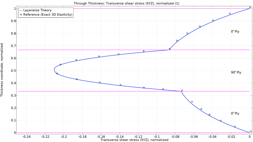
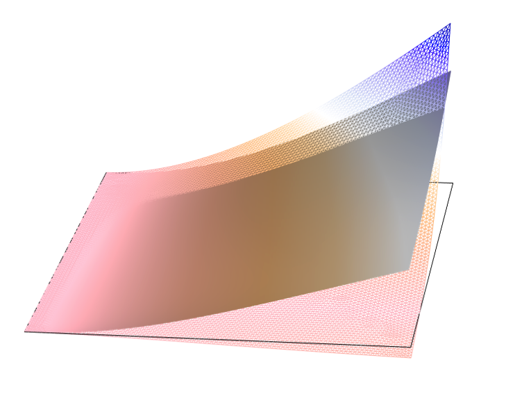
In COMSOL Multiphysics®, the Layered Shell interface is based on the layerwise theory. In the Bending of a Simply Supported Composite Laminate example, a bending analysis of a simply supported composite plate is carried out using the Layered Shell and Shell interfaces. The aim of the analysis is to compare the through-thickness stresses obtained with both interfaces with 3D elasticity solution from a given benchmark.
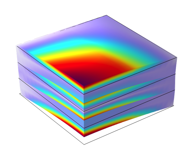
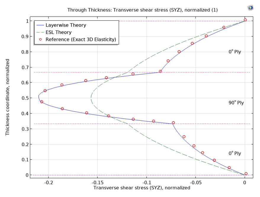
Example of a simply supported composite plate. Left: The von Mises stress distribution in a plate modeled with the Layered Shell interface. Right: A comparison plot of the through-thickness transverse shear stress.
You can also check out the Forced Vibration Analysis of a Composite Laminate to see another example.
Multiple Model Methods: Combination of Shell and Layered Shell Interfaces
The multiple model method is the combination of ESL and layerwise theory applied to different parts of the geometry or layers of composite materials in order to obtain acceptable results with optimal use of computational resources. Apart from the Layered Shell and Shell interfaces, the Layered Shell-Shell Connection multiphysics coupling is needed to couple these two different physics interfaces in the thickness direction.
In the Analysis of a Composite Blade Using a Multiple Model Method example, the Layered Shell and Shell interface are combined to model a composite blade. The aim of the analysis is to compare the solution time of different approaches.
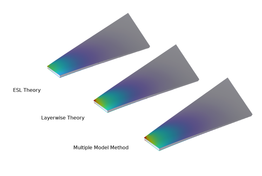
The von Mises stress distribution in a composite blade using different approaches.
Selecting an Appropriate Laminate Theory
Based on the above descriptions, a suitable laminate theory can be chosen. A simple rule of thumb is to choose a laminate theory based on the laminate aspect ratio, which is defined as the ratio of laminate length to the laminate thickness.
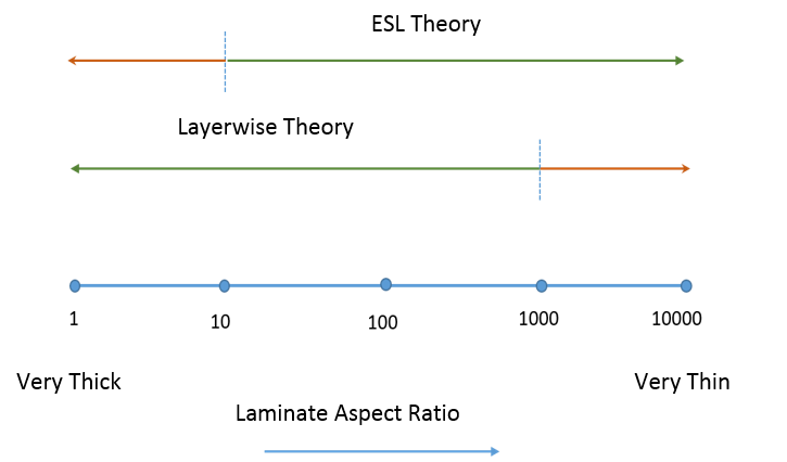
Range of validity for the two laminate theories based on the laminate aspect ratio.
Material Models
The following table lists the material models along with additional inelastic effects available for the analysis of composite materials in different physics interfaces.
| Material Model | Inelastic Effects | Physics Interfaces |
|---|---|---|
| Linear elastic material |
|
|
| Hyperelastic material |
|
|
| Piezoelectric material |
|
|
You can also check out the Pressurized Orthotropic Container — Shell Version and Piezoelectricity in a Layered Shell examples for more details.
Damage, Delamination, and First-Ply Failure Theories
Many composites are quasibrittle materials for which an initial elastic phase is followed by a nonlinear fracture phase after a critical level of stress or strain is reached. As this critical value is reached, cracks grow and spread until the material fractures. The deterioration of material stiffness due to crack growth can be modeled using the Damage feature in the Layered Shell and Shell interfaces. There are two damage models currently available: scalar and Mazar’s. There are also several strain-softening damage evolution laws available. To avoid mesh sensitivity, you can use the spatial regularization method by selecting the Crack Band or Implicit Gradient option.
Delamination, or the separation of layers, is a common failure mode in laminated composite materials. Various factors, including loading, defects in the material, and environmental conditions, can trigger the initiation and propagation of layer separation. To model delamination phenomena, the Delamination feature in the Layered Shell interface can be used. The delamination theory is based on a cohesive zone model (CZM) and there are several traction separation laws included. To learn more, check out the Mixed-Mode Delamination of a Composite Laminate and Progressive Delamination in a Laminated Shell examples in the Application Gallery.
There are several first-ply failure theories available in the Safety feature in the Layered Shell and Shell interfaces. Specifically, theories like Tsai–Wu, Tsai–Hill, Hoffman, Hashin, Hashin–Rotem, Puck, and LaRC03 are useful in composite modeling. To learn more, see the Failure Prediction in a Laminated Composite Shell example.
Buckling
Linear buckling is possible when using either of the two laminate theories; however, ESL-FSDT is more efficient in finding the critical buckling load factor as compared to the layerwise theory. It is possible to optimize a layup in order to maximize the critical buckling load. For more information, see the example Buckling of a Composite Cylinder.
Layered Material Continuity
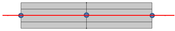
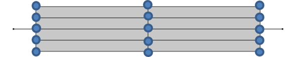
When more than one Single Layer Material or Layered Material Link or Layered Material Stack is active on the selected geometries of the Layered Shell interface, then the DOFs are, by default, disconnected between these different layered materials. The Continuity feature enables you to join two laminates placed next to each other. With this functionality, you can model a ply drop-off scenario. For a modeling example, see Ply Drop-off in a Composite Panel in the Application Gallery.
When using the Shell or Membrane interface, the DOFs are present only on midplanes, thus they are always connected across the layered materials.
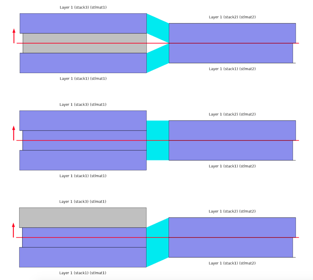
Different ways of setting up the continuity between two laminates placed side by side.
A, B, D Matrix Computation
The standard stiffness and flexibility matrices can be evaluated using the Linear Elastic Material, Layered node in the Shell interface. The four stiffness matrices available are extensional stiffness matrix (A), bending-extensional stiffness matrix (B), bending stiffness matrix (D), shear stiffness matrix (As). You can check out the Material Characteristics of Laminated Composite Shell example for more details.
Sometimes, the material properties of composite laminates are provided in terms of A, B, and D matrices. In such scenarios, the Section Stiffness material feature in the Shell interface can be used.
Results Evaluation Tools for Composite Material Modeling
When performing macromechanics analyses, there are several features in COMSOL Multiphysics® for results evaluation. We discuss some of these features below.
Layered Material Dataset
As the geometry contains only surfaces, the Layered Material dataset is used to display the results of the simulation on a geometry that has a finite thickness. With this dataset, you can scale the laminate thickness in the normal direction, which is useful for thin laminates. The Layered Material dataset also provides an option to perform an evaluation at:
- Mesh nodes
- Interfaces
- Layered midplanes
The Layered Material dataset includes the option to select and deselect different layers of the layered material link or layered material stack. Several other datatsets, like Mirror, Array, Cut Line 3D, Cut Point 3D, and Revolution, can be used with the Layered Material dataset.
Volume and Surface Plots
Different volume plots, surface plots, slice plots, etc., can be used directly with the Layered Material dataset.
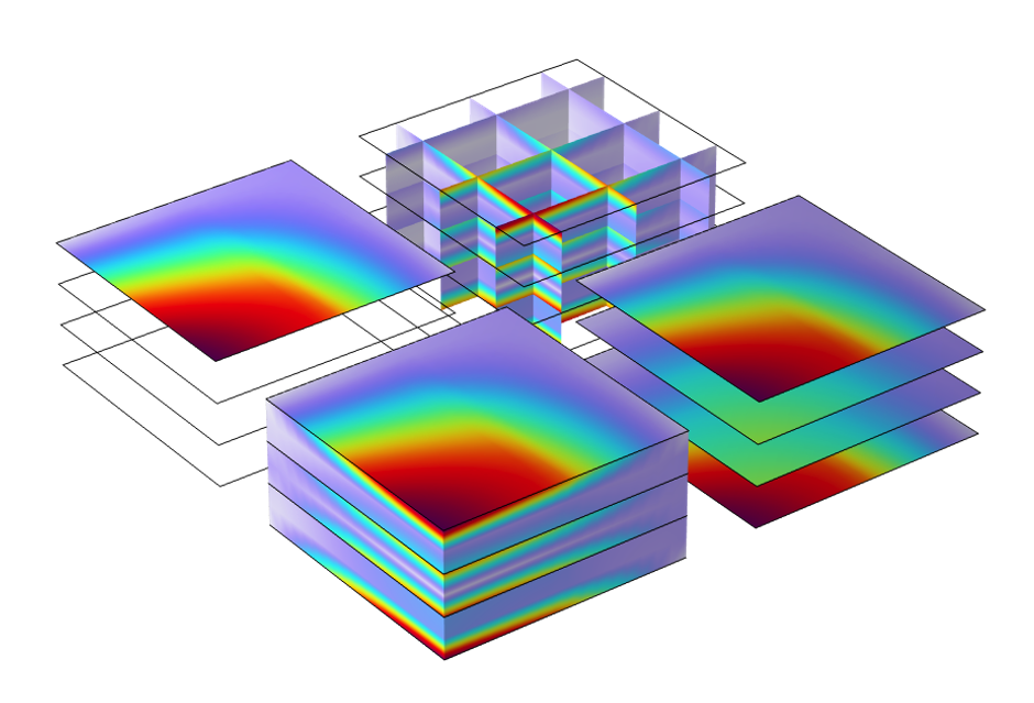
Various plots created using the Layered Material dataset.
Layered Material Slice Plot
For composite laminates, the Layered Material Slice plot offers more freedom when making slices. Some of the instances where this plot is useful include creating a slice:
- Through one (or a couple of) layers
- Through many (or all) of the layers (note that you do not need to place the slices in the through-thickness direction)
- At a certain position in the layer, although not in the midplane
Von Mises stress in the middle of each layer of a laminate, created using the Layered Material Slice plot.
Through-Thickness Plot
This plot is used to determine the variation of different quantities through the thickness of the laminate. You can choose one or several geometric points on the boundary. You also have the option to create a dataset of the cut points as well as to directly enter the point coordinates.
Through-thickness variation of the transverse shear stress at one point in a laminate.
Line or Point Plot
To create a line of a specific variable, you need to use a Cut Line 3D dataset based on the Layered Material dataset. Similarly, to create a point plot of a specific variable, you need to use a Cut Point 3D dataset based on the Layered Material dataset. As an alternative solution, a variable with special operators can be used with either a Layered Material or Solution dataset.
Multiphysics Analyses of a Composite Laminate
Structural Connections
In many scenarios, the structural analysis of a system requires the use of different element types or physics interfaces. The following table lists the multiphysics couplings that can be used to connect the different structural physics interfaces.
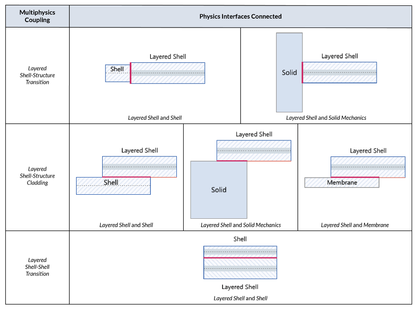
Take a look at the Connecting Layered Shells with Solids and Shells tutorial model to see an example of connecting shell and structural elements.
Thermal Expansion
Thermal expansion in composite structures can be modeled using the following physics interfaces:
- Heat Transfer in Shells
- Shell or Layered Shell
The coupling between different physics is defined using the following multiphysics coupling node:
- Thermal Expansion, Layered
For a modeling example, see Thermal Expansion of a Laminated Composite Shell in the Application Gallery.
Joule Heating and Thermal Expansion
Joule heating and thermal expansion in composite structures can be modeled using the following physics interfaces:
- Electric Currents, Layered Shell
- Heat Transfer in Shells
- Layered Shell
The coupling between different physics is defined using the following multiphysics coupling nodes:
- Electromagnetic Heating, Layered Shell
- Thermal Expansion, Layered
Acoustics–Composite Interaction
Acoustics–composite interaction can be modeled using the following physics interfaces:
- Pressure Acoustics
- Shell or Layered Shell
The Acoustic-Structure Boundary multiphysics coupling node is used to define the interaction between the two physics interfaces.
Fluid–Composite Interaction
This interaction can be modeled using the following physics interfaces:
- Laminar Flow
- Shell or Layered Shell
The Fluid-Structure Interaction multiphysics coupling node is used to define the interaction between the two physics interfaces.
Piezoelectricity–Composite Interaction
Piezoelectricity–composite interaction can be modeled using the following physics interfaces:
- Electric Currents in Layered Shells
- Shell > Piezoelectric Material, Layered or Layered Shell > Piezoelectric Material
The Piezoelectricity, Layered multiphysics coupling node is used to define the interaction between the two physics interfaces. See the Piezoelectricity in a Layered Shell tutorial to learn more.
Piezoresistivity–Composite Interaction
This interaction can be modeled using the following physics interfaces:
- Electric Currents in Layered Shells > Piezoresistive Shell
- Layered Shell
The Piezoresistivity, Layered multiphysics coupling node is used to define the interaction between the two physics interfaces.
Lumped Mechanical Systems–Composite Interaction
This interaction can be modeled using the following physics interfaces:
- Lumped Mechanical Systems
- Layered Shell
The Lumped Structure Connection multiphysics coupling node is used to define the interaction between the two physics interfaces.
Optimization of Composite Laminates
Composite laminates are synthetic structures, and there is always a possibility to optimize a design in terms of the material of each layer, the thickness of each layer, and the stacking sequence. Using the functionality of the Optimization Module, different aspects of a composite laminate can be optimized. To see such optimization, check out the Stacking Sequence Optimization example, in which the stacking sequence of a composite laminate is optimized based on the Hashin failure criterion.
Example of an optimized composite laminate. The displacement in original (wireframe) and optimized (solid) layup.
Multiscale Analysis
Composites can be analyzed at both the macroscale and microscale, and either analysis has its benefits and limitations. Analyses at both the macro and microscale offer an in-depth insight into the composite structure as well as its constituents’ responses to the loading at the macroscale. A full multiscale analysis, which involves macro analysis with micro analysis at each material point, is computationally expensive. If we limit the analysis to only include a few of the critical material points, then we can perform a multiscale analysis by using the Cell Periodicity feature in the Solid Mechanics interface in combination with the Layered Shell interface.
To see a multiscale analysis in action, see the Micromechanics of Failure: Multiscale Analysis of a Composite Structure example. In this example, a micromechanical analysis is first performed to obtain the homogenized material properties, and then a macromechanical analysis using layerwise theory is carried out to obtain the global response. The last step is performing a micromechanical analysis where the local stress and strain field and the failure risk based on the average global strains are computed.
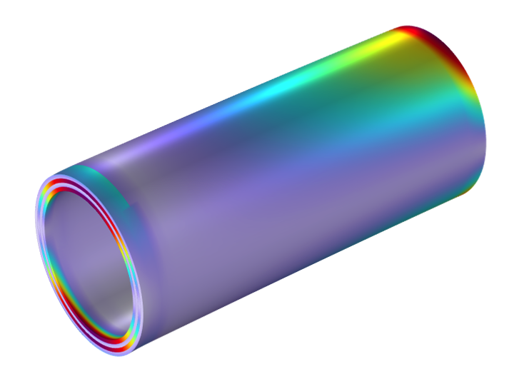
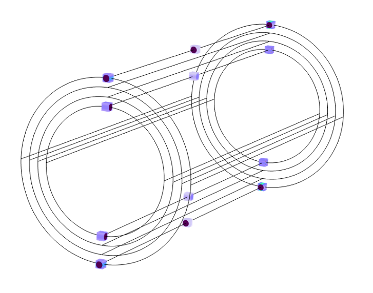
Example of a multiscale analysis. Left: The stress in a composite cylinder based on a macromechanical analysis. Right: The stress at different material points using a micromechanical analysis.
Next Step
With the Composite Materials Module you can design, analyze, and optimize layered composite structures made up of linear or nonlinear materials. To learn more about the Composite Materials Module, contact COMSOL via the button below.


Comments (13)
Dhanunjay
February 26, 2019hello sir,
This is dhanunjay, I am doing micromechanics analysis by representative volume element method and periodic boundary conditions for the fiber of circular and elliptical cross-sections. I am able to perform both separately for different cross-sections if I try to solve in a single file by taking another component and all it is showing only one result and unable to connect the compared graphs between them. But I want both cross-sections to be done in a single file and also need to show the comparison in the form of graphs for the fiber volume fraction and material constants. So in this context, I am seeking your help in performing both RVE models in single file and need comparisons. I hope a positive reply from you. Thanking you very much.
Dhanunjay
February 26, 2019This is my mail id dhanunjayborra@gmail.com and you can send a reply to mail id also. If you want I can send .mph file also. Thank you.
Anonymous
February 26, 2019Dear Dhanunjay,
It is possible to solve for two or more RVE models in a single file but in different components. The only limitation for now is that the homogeneous material created under global definition corresponds to any one of the RVE models. Apart from that, you can plot or derive any quantity from all the RVE models.
If you still face any issues, feel free to send your query and .mph file to support@comsol.com
Best regards,
Pawan Soami
Peter Cendula
January 27, 2021Dear Pawan,
thanks for nice overview. I’m still stuck with version 5.2 at our university and I am wondering if it is possible to calculate bilayer bending by thermal expansion with the Shell interface in 5.2? I tried to add two shells, with one shell being offset by thickness to the other one, but I’m not getting the desired behavior.
Thank you
Peter
Pawan Soami
February 2, 2021 COMSOL EmployeeDear Peter,
Yes, you can simulate bilayer bending by thermal expansion with the Shell interface. As you mentioned, use two shells, place them on top of each other, adjust the offset, connect the DOFs of both shells. I am pretty sure this is something which can be done in version 5.2 also.
If you still face any issues in implementing the above, feel free to send your query and .mph file to support@comsol.com
Best regards,
Pawan Soami
Osama Ahmed
March 20, 2021Hello Sir,
I would like to know if it is possible to model the interaction of elastic waves with delamination in a layered shell, and how can I connect the two physics interfaces
Pawan Soami
March 23, 2021 COMSOL EmployeeDear Osama,
Yes, it is possible to model the interaction of elastic waves with the delamination in layered shell. For this purpose, you don’t need to use Elastic Wave interface. You can model elastic waves within Layered Shell interface. So once you have delamination present in the Layered Shell interface, you can model the interaction of elastic waves with delamination.
Hope this answers your question. If you still face any issues in implementing the above, feel free to send your query and .mph file to support@comsol.com
Best regards,
Pawan Soami
Vibhu Khantwal
September 20, 2023Hello Sir,
Can we do ablation modeling on composite materials? for eg. material removal due to laser or due to some heat flux. if yes, how we can do that. what are the commands should i follow.
thankyou
Amit Suresh Patil
January 26, 2024 COMSOL EmployeeDear Vibhu,
For such modeling you need a Deformed Geometry interface and Solid Mechanics interface to model the composite material rather than the Layered Shell interface. There is a blog post about it, please have a look.
https://www.comsol.com/blogs/modeling-thermal-ablation-for-material-removal/
If you still face any issues in implementing the above, feel free to send your query and .mph file to support@comsol.com
Said Bouta
January 25, 2024Dear Peter,
Can you help me how can to add periodic boundary condition PBC in the case of RVE wit matrix elastoplastic.
Amit Suresh Patil
January 26, 2024 COMSOL EmployeeDear Said,
The periodic boundary conditions would remains the same for elastoplastic material. The important question is what is the purpose of applying PBCs. In above blog post we have shown how to extract the homogenized elastic properties using the PBCs for elastic material. You can use the PBCs to extract the homogenized yield stress (by adjusting macroscopic strain values and using different loadcases), you can use PBCs to get the response of elastoplastic periodic materials after yielding (see the research paper: Apparent elastic and elastoplastic behavior of periodic composites).
For further questions, feel free to send your query and .mph file to support@comsol.com
Best Regards,
Amit
Garshasp Keyvan Sarkon
January 28, 2024Subject: Error in Plotting Datasets in Layered Shell Interface Simulation
Dear Mr. Patil and COMSOL Technical Team,
I am currently working on a tensile test simulation using the layered shell interface in COMSOL, and I have encountered a persistent issue that I hope you can assist me with.
For the sake of efficiency in simulation runs, I chose to model my geometry as a 2D rectangle, while applying 3D physics (layered shell interface). However, I am facing a consistent error when I attempt to define and use 1D, 2D, or 3D plot datasets in their respective plot groups. This error is proving to be a significant roadblock in my analysis.
I am beginning to wonder if this problem might have been avoided if I had initially defined a 3D block instead of a 2D rectangle. Could this change in the geometric definition be the solution to the plotting issues I am facing?
I would greatly appreciate any tips, insights, or guidance you can provide to help resolve this issue. Your expertise in this matter would be invaluable to my project.
Thank you for your time and assistance.
Best regards,
Gary
Amit Suresh Patil
January 28, 2024 COMSOL EmployeeDear Garshasp,
You are correct to use the 2D geometry with the Layered Shell interface. From your question it is not clear which datatsets you are working with. The Layered Shell interface predominately needs a Layered Material dataset to work with, although there is a way to work with a Solution datatset. We would able to provide you a quick support if you send your query and mph file to support@comsol.com
Best Regards
Amit