support@comsol.com
Studies and Solvers Updates
COMSOL Multiphysics® version 6.1 provides better performance for CFD simulations and for the Adaptive Frequency Sweep study step. The Adaptive Mesh Refinement study settings have been reorganized and now come with a new setting for saving disk storage space. Browse all of the updates below.
Improved Performance for CFD
The symmetrically coupled Gauss–Seidel (SCGS) method, used by many CFD applications, has been improved with better default settings. In many cases, this provides a 30% reduction in CPU time. Furthermore, the memory requirement for multigrid solvers with cluster computing has been reduced by up to 25%.

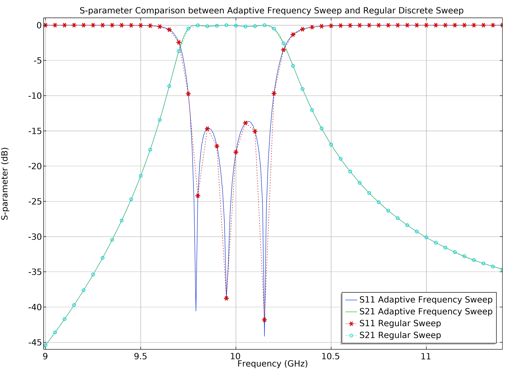
Improved Performance for Adaptive Frequency Sweep
The Adaptive Frequency Sweep study step has been optimized for analyses in which the field output is stored only for a selection, such as a domain or boundary. This is useful for ports in filter applications, for example. The performance improvement for such a sweep is up to 25%. The performance gain is even greater for applications where very high resolution results are required. The following models showcase this new improvement:
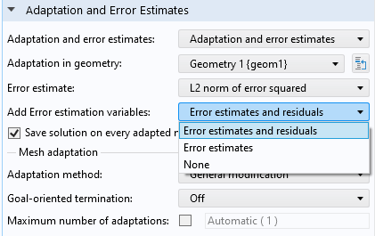
Improvements to Adaptive Mesh Refinement
The most important settings for adaptive mesh refinement can now be found at the study level for all study types that support this functionality. Furthermore, you can substantially save disk storage and memory requirements for the Functional and L2 norm of error squared error estimate methods. You can do so by selecting the None option (see screenshot), which means that no error estimation or residuals are added.
Sensitivity Analysis for Eigenvalue Problems
It is now possible to use an Eigenfrequency or Eigenvalue formulation in Sensitivity analyses. With this extended functionality, you can now perform gradient-based optimizations where the objective or constraints depend on the eigenvalue from these formulations. In structural mechanics, for example, this functionality can be used to investigate an eigenfrequency’s sensitivity to input parameters. View this update in the Maximizing the Eigenfrequency of a Shell model.
Explicit Methods for Time Stepping for Solving DAEs
Explicit time-stepping methods can now be used to solve differential-algebraic equations (DAEs). Such systems are found in, for example, elastic wave propagation problems in solid mechanics. For the Time-Dependent Solver, we have introduced Implicit and Explicit solver types. All methods previously available from the Time-Explicit Solver are now listed in the Method drop-down menu when you select Explicit as the Solver type. The previous Time-Explicit Solver has been removed but is still available for models built in earlier versions of the software.
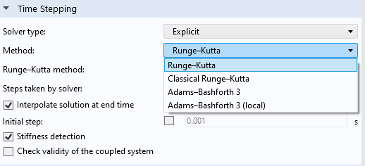
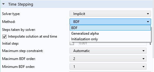
The new Solver type settings for the Time-Dependent Solver.