Particle Tracing Module Updates
For users of the Particle Tracing Module, COMSOL Multiphysics® version 5.3a brings a new null collision method for colliding particles, random particle release times, and a new benchmark tutorial model. Browse all of the new features and functionality in the Particle Tracing Module below.
Null Collision Method
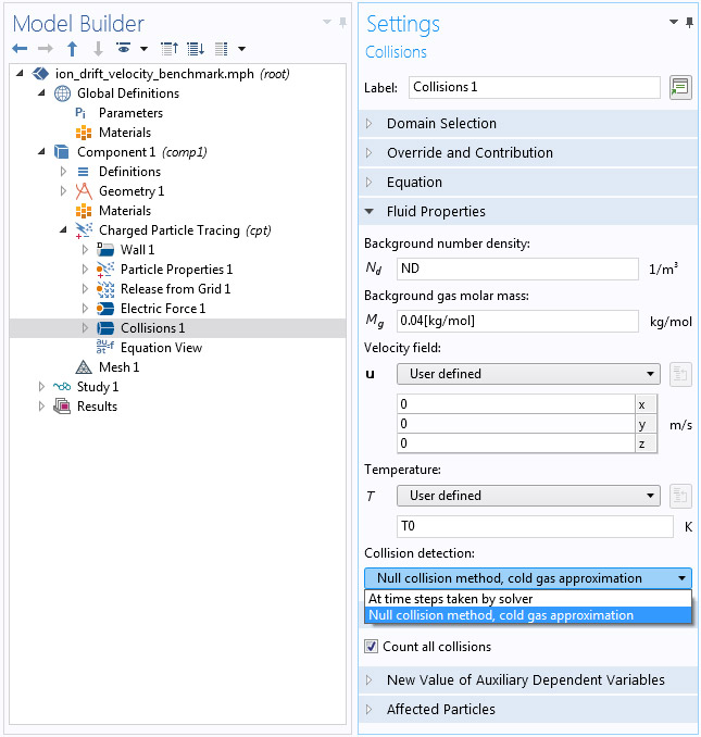
The Collisions feature for the Charged Particle Tracing interface now supports a null collision method for Monte Carlo modeling of the interaction between ions, electrons, or molecules with a rarefied gas. The null collision method is capable of modeling multiple collisions for each particle within a single time step taken by the solver. It also has limited capabilities to account for variations in the collision frequency within the time step. This method provides the greatest benefit to simulations of energetic particles, with speeds much greater than the thermal velocity of the background gas.
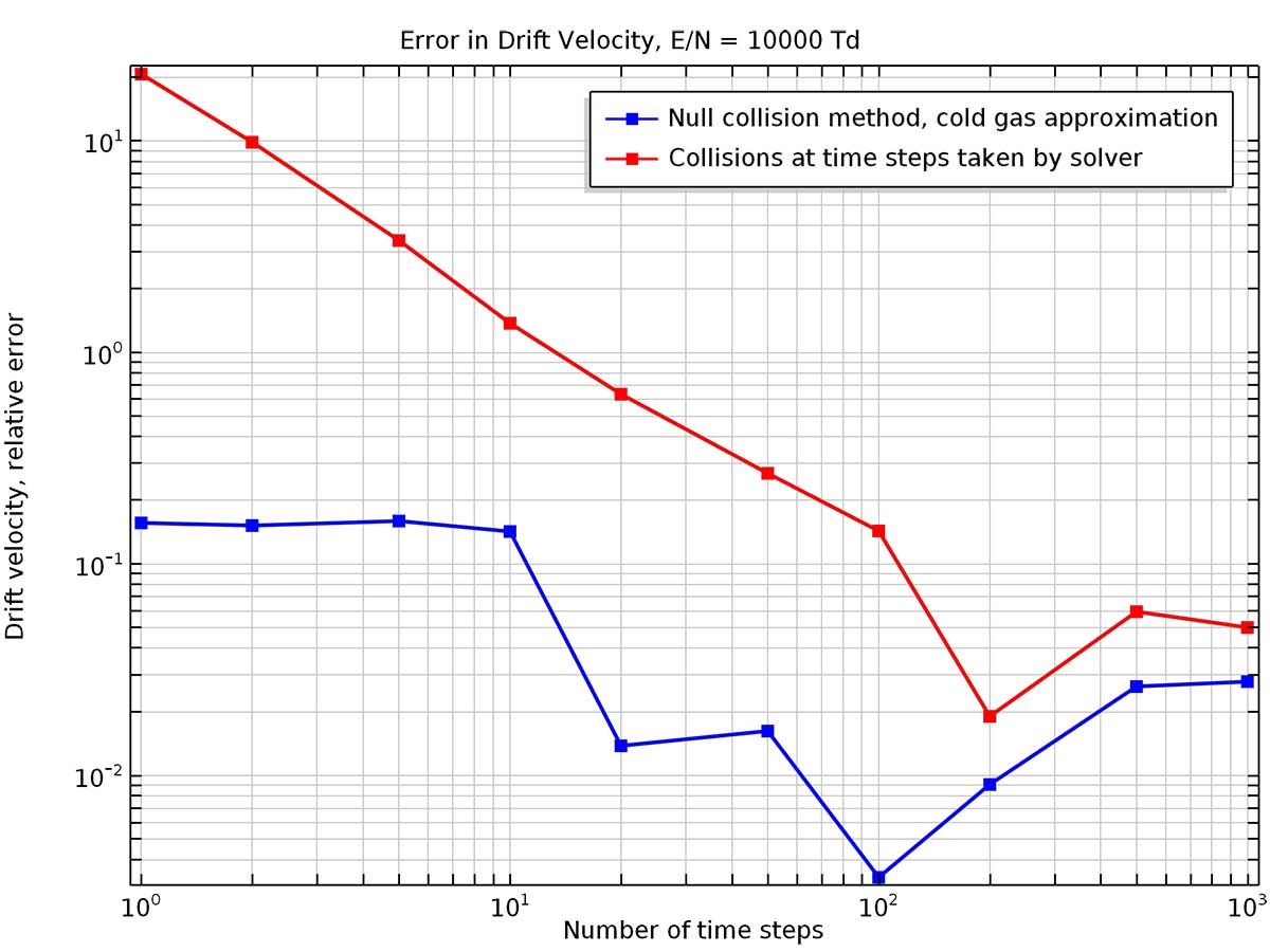 Relative error of the Ion Drift Velocity Benchmark model for different manual time step sizes. In this example, the null collision method is consistently the more accurate collision detection algorithm, but the difference is most noticeable for large time steps.
Random Particle Release Times
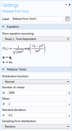
In addition to specifying a list of particle release times, you can now select a uniform, normal, or lognormal distribution of particle release times, which can either be random or deterministic. The normal distribution, for example, allows more particles to be released closer to the mean release time and fewer particles at time values far away from the mean release time.
Particles are released at random locations at the inlet for a normal distribution of release times. The color represents the time from the mean release time (red particles are released closer to the mean release time and blue particles farther from the mean). As expected, more particles are released close to the mean release time.
Reuse Disappeared Particles for Secondary Emission
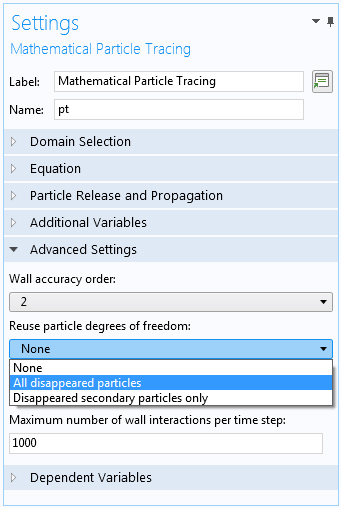
In models with secondary particle emission, you can now recycle degrees of freedom from particles that have disappeared earlier in the study. This saves a considerable amount of memory in models where particles get created and annihilated many times in rapid succession.
More Flexible Periodic Electric and Magnetic Forces
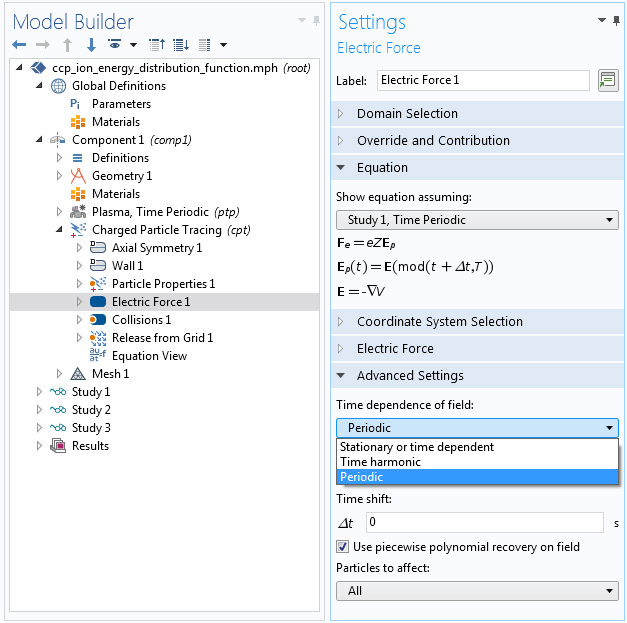
You can now define electric and magnetic forces that are periodic, but not time harmonic. In the settings for the Electric Force or Magnetic Force nodes, select Periodic from the Time dependence of field list. With this new functionality, if you run a transient simulation to compute the electric or magnetic field over one period, you can then easily trace particles in the field for arbitrarily many periods.
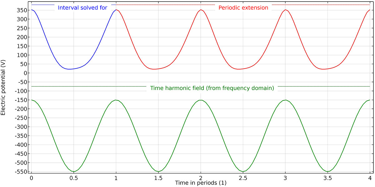
In plasma simulations, the electric potential is often periodic, but not time harmonic. Above is the potential from the tutorial CCP Ion Energy Distribution Function, which requires the Plasma Module, and a time harmonic potential for comparison. The new settings for periodic electric and magnetic forces are more compatible with such general periodic fields.
Application Library path:
Plasma_Module/Capacitively_Coupled_Plasmas/ccp_ion_energy_distribution_function
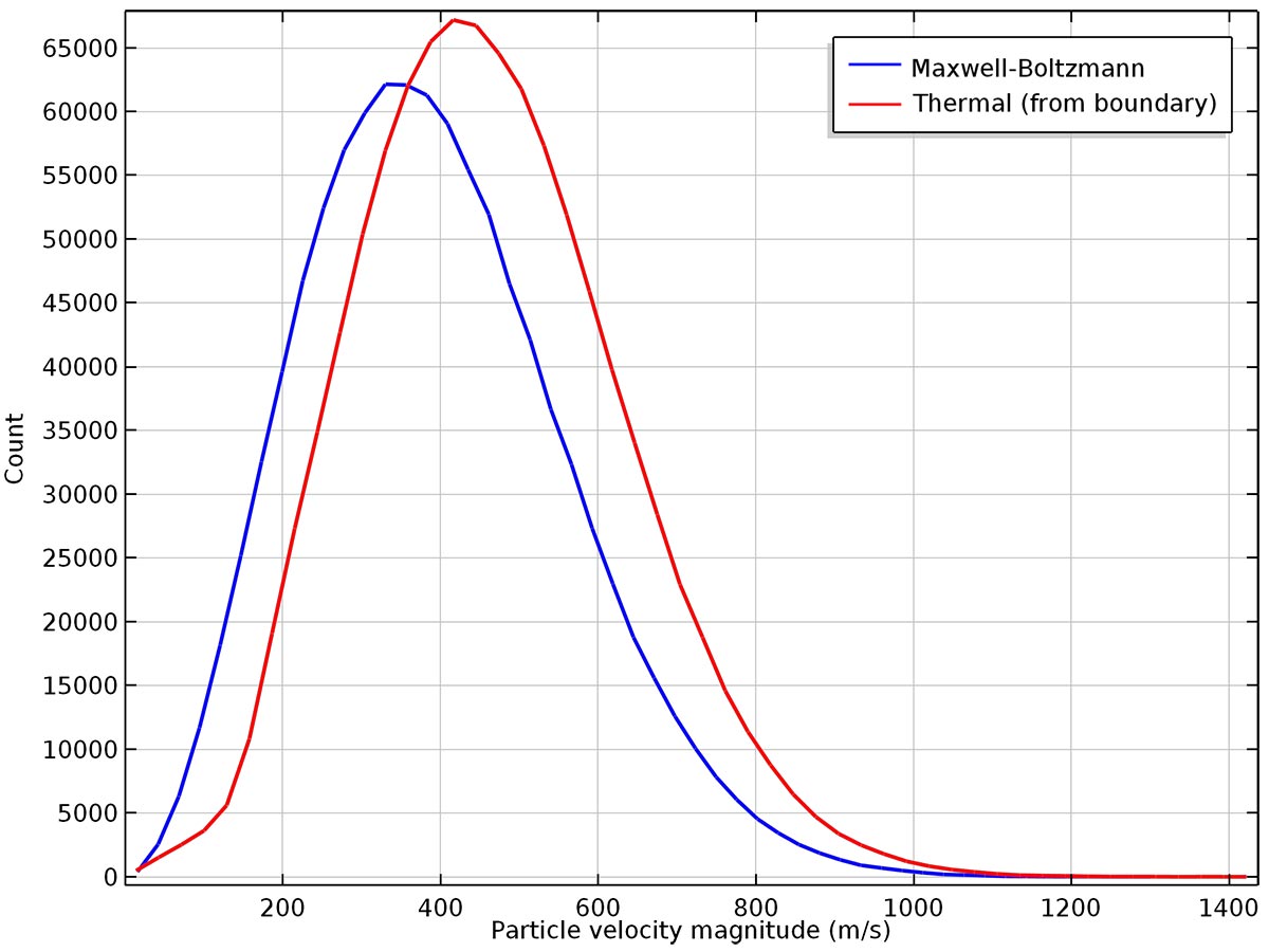
Thermal Distribution of Particle Velocities from Boundaries
You can now release particles or reinitialize particle velocity at a boundary by sampling their speeds from a thermal distribution based on wall temperature. Unlike other available particle-wall interactions, such as the diffuse or specular reflection, the new Thermal Re-Emission boundary condition samples the particle speed from a distribution, not just the direction of the velocity vector.
Two variants of this feature are available. Use the Thermal velocity distribution, available with the Inlet feature, to sample released particle speeds from the distribution. Alternatively, use the Thermal Re-Emission wall condition to model molecules that get adsorbed at the boundary and then immediately reemitted into the domain with different speeds based on the surface temperature.
Animation of molecules being adsorbed and reemitted at a surface.
Grid-Based Release with Cylindrical and Hexapolar Coordinates
You can now release particles from a cylindrical or hexapolar grid of points when using the Release from Grid feature. You can control the center and orientation of the cylindrical distribution, the number of different radial positions, and the number of angles.
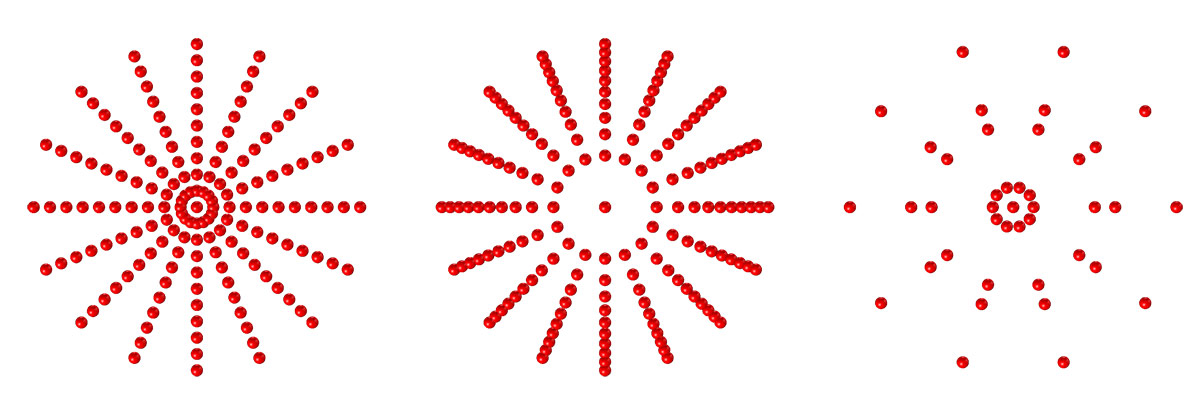
Cylindrical grid-based distributions can be specified with uniform gaps between rings of grid points (left), gaps scaled to approximate uniform spatial number density (middle), or user-defined radii (right).
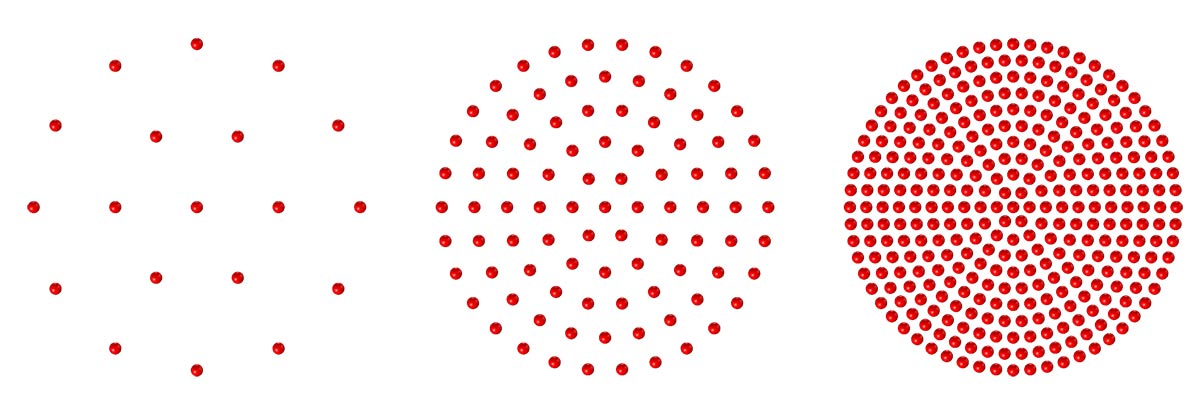
From left to right: Hexapolar grids containing two, five, and ten rings of points.
New Benchmark Model: Particle Dispersion in a Turbulent Channel Flow
This tutorial model demonstrates some of the phenomena that occur when particles move through a turbulent channel flow. The fluid velocity is computed using a Reynolds-Averaged Navier-Stokes (RANS) model and, as a result, the individual eddies of the flow are not explicitly modeled. To couple such a flow field to the particle tracing simulation and still account for turbulent dispersion, a continuous random walk (CRW) model is used. The CRW model perturbs the drag force on the particles in random directions based on the turbulent kinetic energy and turbulent dissipation rate of the fluid.
This example shows how inhomogeneous, isotropic turbulence in the wall region affects the particle motion. Particles of sufficiently high inertia tend to cluster close to the wall because of their ability to cross between different eddies in the flow. To show how the particle inertia affects the distribution of particles downstream in the channel, a Parametric Sweep is run over six different values of the Stokes number. The results are compared to direct numerical simulation (DNS) data from the published literature.
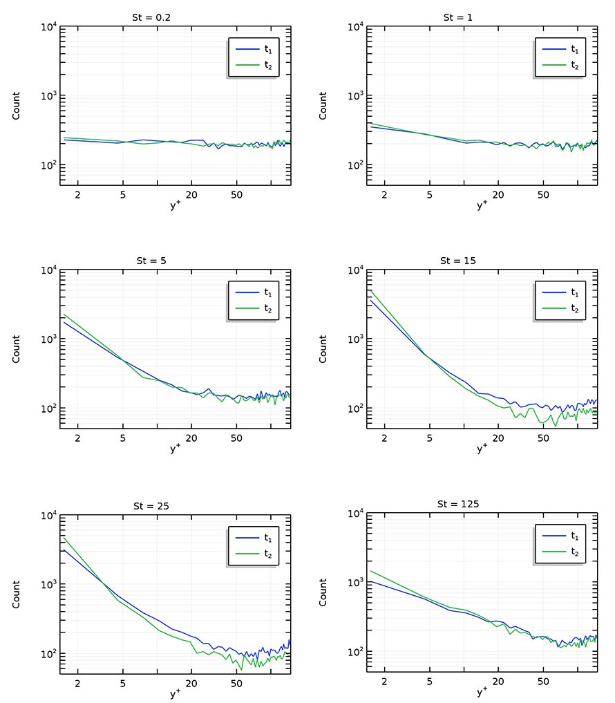
Histograms of particle position in viscous units. Smaller values of y+ correspond to positions closer to the channel walls.
Application Library path:
Particle_Tracing_Module/Fluid_Flow/flow_channel_turbulent_dispersion