CFD Module Updates
For users of the CFD Module, COMSOL Multiphysics® version 5.3a includes a new realizable k-ε turbulence model, buoyancy-induced turbulence, and an inlet boundary condition for fully developed turbulent flow. Browse these and more CFD Module updates below.
New Realizable k-ε Turbulence Model Interface
The new Turbulent Flow, Realizable k-ε interface adds a popular RANS turbulence model to your arsenal of turbulence models. Most turbulence models include realizability constraints to ensure nonnegativity of turbulent normal stresses, Schwarz's inequality between any fluctuating quantities, and to limit the production of turbulence. However, the new realizable k-ε turbulence model applies realizability by allowing the coefficients in the turbulence transport equations to vary with respect to the mean flow deformation rate as well as k and ε. This results in a smoother, more physical approach to the limiting states.
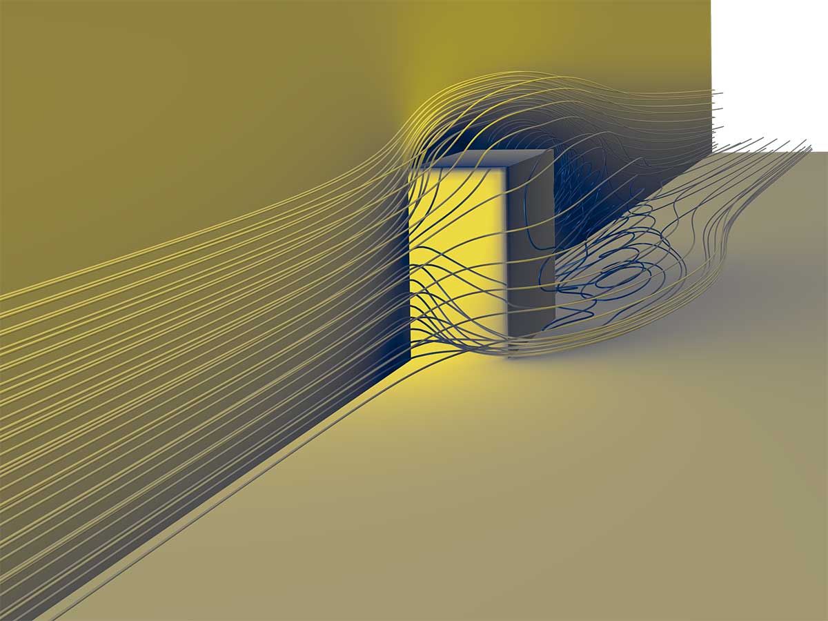 Turbulent flow hitting a cube at a straight angle to one of the faces. The realizable k-ε turbulence model prevents the turbulent energy component in the strain direction from assuming negative values due to rapid mean strain.
All Turbulence Models Now Available for Rotating Machinery
The new version of the CFD Module contains ready-made formulations for all of the turbulence models when used in tandem with rotating machinery. This makes it simpler to model turbulent flow with rotating machinery for any turbulence model that previously had to be defined manually, in a rotating frame.
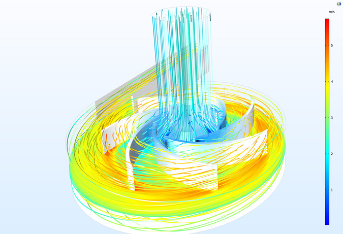 Model of a centrifugal pump modeled with the new turbulence model and rotating machinery combination.
All Turbulence Models Now Available for the Mixture Model and Bubbly Flow Interfaces
The Bubbly Flow and Mixture Model interfaces now include all turbulence models as well as automatic wall treatment, except the inherently wall-law-based k-ε and realizable k-ε formulations. Additionally, interior wall boundary conditions are available, thus making it possible to treat impellers, rotors, baffles, fins, etc. without having to mesh thin walls.
Benchmark model of turbulent bubbly flow, also making use of bubble-induced turbulence. The animation shows the volume fraction of bubbles with a view from below.
Buoyancy-Induced Turbulence
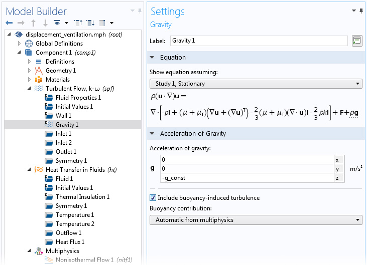
Buoyancy introduces a volume force in the bulk of a fluid that may naturally cause instabilities. Eventually, these instabilities in the flow become chaotic, leading to the onset of turbulence. The Gravity feature, used for modeling buoyancy in the CFD Module, now includes the option of accounting for buoyancy-induced turbulence by selecting the corresponding check box. This contribution to the turbulent flow can then be defined either automatically from the Nonisothermal Flow multiphysics coupling or from a user-defined turbulent Schmidt number.
Inlet Boundary Condition for Fully Developed Turbulent Flow
The Inlet boundary condition for fully developed turbulent flow gives the velocity profile and the turbulence variable values at an inlet cross section, assuming that the inlet channel upstream is of a certain length and that the flow is fully developed. In previous versions of the COMSOL® software, a decent estimate of the cross section velocity profile would have required modeling a very long inlet section of the channel. The new boundary condition gives a very accurate inlet profile without the need for extra geometry and therefore reduces the computational resources.
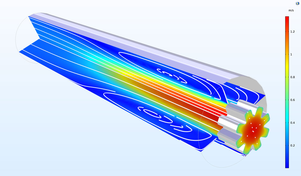 The inlet from a nozzle with star-shaped cross section is modeled using the fully developed turbulent flow inlet condition.
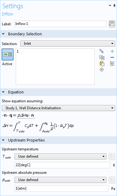
New Boundary Condition: Inflow
The new Inflow boundary condition applies an inflow of heat coming from a virtual domain, which has been excluded from the model to simplify the analysis, with known upstream conditions. Applied at inlets, where you would previously apply a Temperature boundary condition, the Inflow condition accounts for temperature and pressure from upstream phenomena. Additionally, it does not constrain the temperature at the inlet's adjacent edges (or points in 2D), but instead assigns a heat flux that is consistent with the upstream conditions. Overall, this leads to more accurate and realistic physical models. All the applicable models in the Application Libraries have been updated to take advantage of this boundary condition.
Revamped Rotating Machinery Interfaces with Moving Mesh
The Rotating Machinery, Fluid Flow interfaces have been improved by separating the Rotating Domain node from the fluid flow physics. When adding one of these interfaces, the single-phase flow interface is added as well as a Rotating Domain node under Definitions > Moving Mesh. With this separation, you can now combine any fluid flow interface with rotating machinery. Even with this increased flexibility, it is just as easy to define fluid flow in rotating machinery and the separate moving mesh as with previous versions of COMSOL Multiphysics®. The moving mesh controls the spatial frame in a model and may apply to all physics interfaces in a model where the domains are rotating. As an example, this simplifies the combination of fluid flow with chemical species transport in mixers and stirred reactors.
The tutorial model of a gently mixed liquid solution utilizes the new rotating machinery interface for laminar flow. The rotating machinery interface is also available for all turbulence models for more vigorously stirred mixers and tank reactors.
New Fluid-Structure Interaction Interface That Supports All Turbulence Models
A new Fluid-Structure Interaction multiphysics coupling has replaced the interface used in previous versions of the COMSOL® software. The new coupling matches the modern style, with a number of single-physics interfaces and multiphysics nodes to couple them together. With this approach, all functionality in the constituent physics interfaces is available for fluid-structure interaction (FSI) modeling. On the structural side, many additional boundary conditions and material models are now available for FSI analysis; for example, rigid domain, piezoelectric, and nonlinear elastic material models. On the fluid side, all turbulence models are now available as well as a number of new boundary conditions. After adding a Fluid-Structure Interaction interface from the Model Wizard, you will get a Solid Mechanics interface, a Laminar Flow interface, a Fluid-Structure Interaction multiphysics coupling node, and a Moving Mesh node in the Definitions section. All fluid-structure interaction models in the Application Libraries have been updated to include this new coupling functionality.
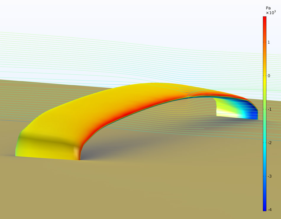 Pressure (color table) and deformation (exaggerated by a factor of 50 at the surface) of a sports car wing subjected to turbulent flow (streamlines) of 200 km/h (125 mph) in a test bench. The model is defined using one-way fluid-structure interaction in the new physics interface.
Substantially Improved Performance and Stability for Time-Dependent Problems
The solver strategy for time-dependent problems has been modified, resulting in a smoother and more robust solution process that is up to 50% faster without losing any accuracy.
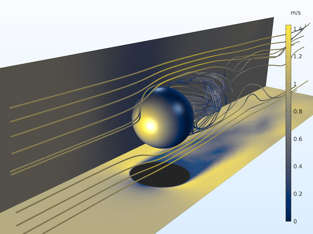 Time-dependent model of the flow around a sphere creating a Karman vortex street downstream, solved more quickly in COMSOL Multiphysics® version 5.3a.
Revamped Free and Porous Media Flow Interface
With the new version of the Free and Porous Media Flow interface, you can couple laminar or turbulent free flow with porous media flow. This interface remains unique in its coupling with the electrochemistry interfaces for the modeling of porous electrodes.
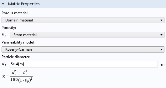
Kozeny-Carman Permeability Model
The Kozeny-Carman permeability model, available for the Darcy's Law interface in COMSOL Multiphysics® version 5.3a, allows you to estimate the permeability of granular media from the porosity and particle diameter.
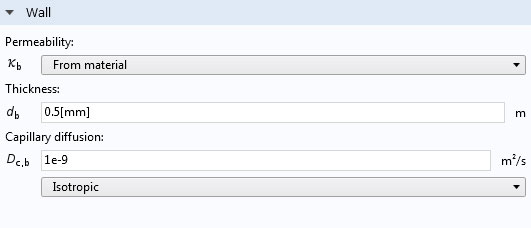
Thin Barrier Feature in the Two-Phase Darcy’s Law Interface
The Two-Phase Darcy’s Law interface can now be used to define permeable walls on interior boundaries. These interior boundaries are used to represent thin, low-permeability structures. The Thin Barrier feature avoids expensive meshing of thin structures, such as geotextiles or perforated plates. Additionally, the permeability of the interior wall can be either isotropic or anisotropic.
New Tutorial Model: Flow in a Hydrocyclone
The v2-f turbulence model introduced in the last release of COMSOL Multiphysics® is well suited for the modeling of hydrocyclones, giving highly accurate results. Therefore, we have included this tutorial model to help you implement such a turbulence model in your own designs. The results show the velocity field and pressure drop in the hydrocyclone, both of which are in very good agreement with scientific literature.
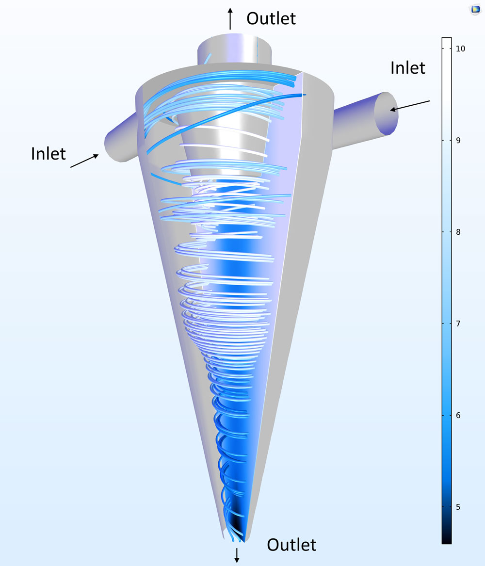 Flow and particle trajectories in a hydrocyclone. The lighter particles are entrained in the flow and follow the main flow upwards to the upper outlet. The heavier particles are expelled radially outwards due to the centrifugal force and exit together with a small fraction of the flow through the lower outlet.
Application Library path:
CFD_Module/Single-Phase_Tutorials/hydrocyclone
New Tutorial Model: Acoustic Liner with a Grazing Background Flow
This model demonstrates how to compute the acoustic properties of an acoustic liner with a grazing flow. The liner consists of eight resonators with thin slits and the background grazing flow is at Mach number 0.3. The sound pressure level above the liner is computed and can be compared to results from a published research paper. The model first computes the flow using the SST turbulence model available in the CFD Module. The acoustics are then computed using the Linearized Navier-Stokes, Frequency Domain interface of the Acoustics Module.
Note that the CFD Module is needed to run this model.
Application Gallery link:
Acoustic Liner with a Grazing Background Flow
New Tutorial Model: Coriolis Flow Meter
A Coriolis flow meter, also known as a mass flow meter or an inertial flow meter, is used to measure the mass flow rate of a fluid traveling through it. It makes use of the fact that the fluid's inertia through an oscillating tube causes the tube to twist in proportion to the mass flow rate. Typically, the density and thereby the volumetric flow rate can also be assessed using the device.
This model shows how to simulate a generic Coriolis flow meter with a curved geometry. When the fluid passes through the elastic structure, a curved duct, it interacts with the movement of the duct when vibrating. The phase difference between the deformation of two points on the duct is caused by the Coriolis effect and can be used to evaluate the mass flow rate through the system.
This model uses the Linearized Navier-Stokes, Frequency Domain interface coupled to the Solid Mechanics interface using the built-in multiphysics coupling. The background mean flow is modeled using the Turbulent Flow, SST interface. In this way, fluid-structure interaction (FSI) can be modeled efficiently in the frequency domain.
Movement of the Coriolis flow meter pipe for three mass flow rates. The flow meter is actuated at the natural frequency of the structure. The deformation amplitude and phase are exaggerated for visualization. As the flow rate increases, the phase difference upstream and downstream increases.
Application Gallery link:
Coriolis Flow Meter: FSI Simulation in the Frequency Domain