
One of the more common questions we get is: How large of a model can you solve in the COMSOL Multiphysics® software? Although at some level this is a very easy question to answer, it inevitably leads to a longer conversation about numerical methods, modeling strategies and solution algorithms, and computer hardware performance, as well as how to best approach computationally demanding problems. Let’s take a deeper dive into this topic.
Editor’s note: The original version of this post was published on October 24, 2014. It has since been updated to reflect new features and functionality.
Let’s Look at Some Data
We will start by setting up a three-dimensional model for the steady-state temperature distribution within a domain and study the memory requirements and solution time with an increasing number of degrees of freedom (DOFs). That is, the model is solved on successively finer and finer meshes while using the default solver on a typical desktop workstation machine — in this case, an Intel® Xeon® W-2145 CPU, with 32 GB RAM, and a solid-state drive (SSD).
We will first look at the memory requirements as the model size is increased in terms of two reported quantities: the virtual memory and the physical memory. The virtual memory is the amount of memory that the software is requesting from the operating system (OS). (These data are from a Windows® machine, and memory management on all supported OS’s is very similar.) The physical memory is the amount of RAM memory that is being occupied. Physical memory will always be less than both virtual memory and the amount of installed RAM, since the OS, as well as other programs running on the computer, will also need to occupy some fraction of the RAM. There is a point where the available space in the physical RAM is used up, and a significant fraction of the data resides on the SSD. There is also a point beyond which the software will report that there is not enough memory, so the model cannot be solved at all. Clearly, adding more memory to our computer would let us solve a larger model, and we can linearly extrapolate to predict the memory requirements.
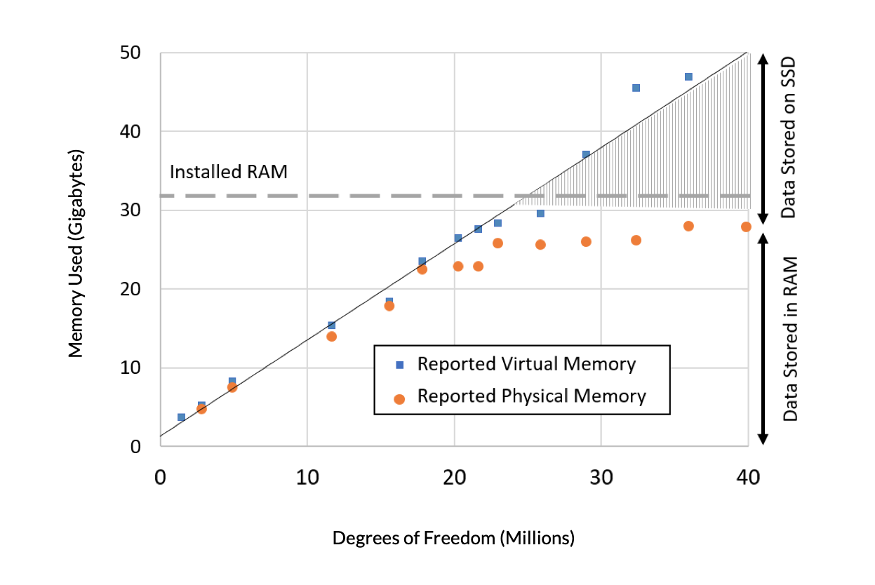
Figure 1. Reported virtual memory (blue) and physical memory (orange) needed versus problem size, in terms of millions of DOFs, for a model involving heat transfer in solids. A computer with 32 GB RAM was used.
Next, let’s look at the solution time for this problem versus, again, the degrees of freedom. The solution time exhibits two distinct regions. A second-order polynomial is fit to the region where the amount of virtual memory needed is less than the installed RAM, and this curve is nearly linear. Another second-order polynomial is fit to the remaining data, where the virtual memory is higher than the installed RAM. This exhibits a steeper slope since in this regime it takes longer to access the model data stored in virtual memory.
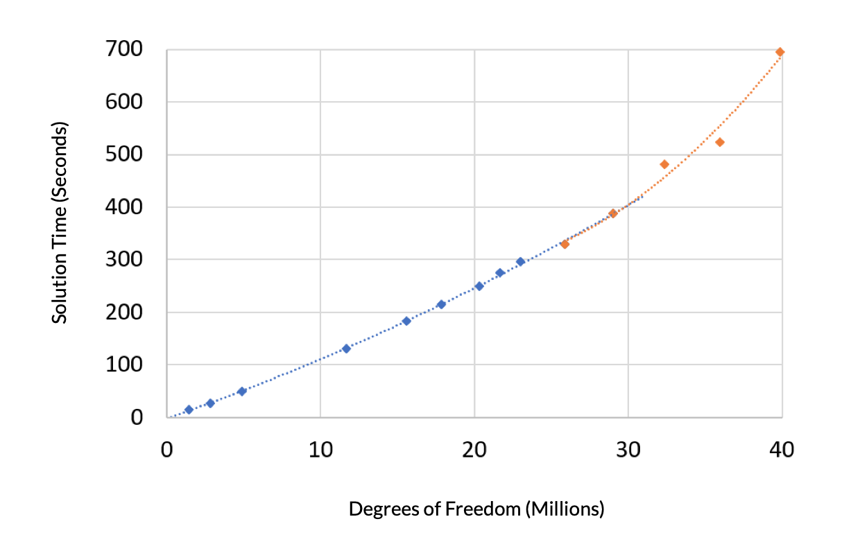
Figure 2. Solution time versus DOFs exhibits an increased slope when the problem size is larger than the available RAM.
Will the Memory Requirements Always Be the Same?
We can reasonably ask whether the preceding data about memory requirements will always be true. As you’ve probably surmised, the answer is no, the data has very little predictive value other than for very similar problems.
6 Typical Modifications Made to Models
What are some of the common changes that we could make to the current model that will cause these curves to shift up or down? We cover several different examples below.
1. Solving in the Time Domain
Solving a problem in the time domain, using a Time-Dependent solver, will require storing more data in memory as compared to solving a steady-state problem. For an overview of the algorithms, read our blog post “Automatic Time Step and Order Selection in Time-Dependent Problems”.
2. Switching the Linear Solver Type
The aforementioned problem could be solved with either iterative or direct solvers. Iterative solvers will use significantly less memory than direct solvers, especially as the problem size grows. Direct solvers are warranted only for certain problem types, such as when the system matrix is nearly ill-conditioned due to high contrasts in material properties, for example, but still scales superlinearly.
3. Introducing a Nonlinearity
Even within a single physics, introducing any kind of nonlinearity, such as making the material properties a function of temperature, can result in the system matrix being nonsymmetric. This will increase the memory requirements. It’s possible to prevent this by using the nojac() operator to avoid symbolic differentiation, although that is not desirable to do in all cases, since it may negatively affect the nonlinear convergence rate.
4. Changing the Element Type
The default element type for a three-dimensional problem is the tetrahedral element, but another element type could also be used, such as a triangular prismatic or hexahedral. These elements have greater connectivity per element and will increase memory usage. On the other hand, switching element types can be strongly motivated for certain geometries and problem types, since they can lead to much coarser meshes for the same geometry, especially when combined with geometry partitioning and swept meshing.
5. Changing the Element Order
The default element order when solving for Heat Transfer in Solids is the quadratic Lagrange. Changing to linear will decrease the number of degrees of freedom in the model if the mesh is the same and will also lead to each element having less connectivity. That is, each node within each element has fewer neighboring nodes to communicate with. This leads to a lower memory usage for the same DOFs. On the other hand, increasing element order leads to greater connectivity, which leads to higher memory usage for the same DOFs. Furthermore, one can switch between Lagrange and serendipity elements, the latter having less nodes per element. It’s necessary to understand, however, that changing the element order and type has effects on both accuracy and geometry meshing requirements, which is a complicated topic on its own, so changing element order from the default should be approached with care.
6. Introducing Nonlocal Couplings or Global Equations
A nonlocal coupling involves any kind of additional coupling terms that pass information between non-neighboring elements and are often used in conjunction with global equations. Using these affects the amount of information in the system matrix and often makes the problem nonlinear. There are certain boundary conditions, such as the Terminal boundary condition, that are available for problems involving electric currents and introduce nonlocal couplings or global equations behind the scenes. Nonlocal couplings can also be manually implemented as discussed in our blog post “Computing and Controlling the Volume of a Cavity”.
Solving for Different Physics
Now, what about if you’re solving different physics? The abovementioned example related to the modeling of heat transfer, where the finite element method (FEM) is used to solve for the (scalar) temperature field. If you are solving a different physics via the FEM, then you might instead be solving for a vector field. For example:
- Solid Mechanics
- The Solid Mechanics interface solves for the displacement field in 3D space, so for the same mesh there will be three times as many degrees of freedom, and more connectivity between them, as compared to the thermal problem. For some solid mechanics problems involving incompressible solids, additionally solving for the pressure will increase memory requirements even more. Introducing nonlinear material models can further increase memory requirements depending on the material models being used.
- Fluid Flow
- The Fluid Flow interfaces all solve for the velocity field in 3D, as well as pressure. When solving for turbulent flow, at least one additional turbulence variable is solved for. When solving for multiphase flow, there is at least one additional variable that tracks phase.
- Electromagnetics
- Depending on what governing equations you’re interested in, you might be solving either a scalar equation or vector equation, or even adding an additional gauge fixing equation.
- Chemical Species Transport
- When solving chemical engineering problems, such as reacting flows, the number of degrees of freedom is proportional to the number of chemical species that you are including in the model.
Keep in mind that for each of these physics, or any other solved via FEM, we again have to consider the effect of all of the previously mentioned points. And what about if we look beyond FEM? There are interfaces and methods within COMSOL® that we can use, such as the Particle Tracing interface, which solves a set of ordinary differential equations (ODEs) for particle position and has much lower memory requirements versus degrees of freedom compared to FEM; the Ray Optics interface, which also solves a set of ODEs and has similar memory requirements as particle tracing; the discontinuous Galerkin (dG) approaches — which are used for solving electromagnetic wave, acoustic, and elastic wave models — use very little memory compared to FEM; and, lastly, the boundary element method (BEM), which is a discretization method, but of boundaries rather than volumes. This leads to much higher memory requirements for each degree of freedom compared to FEM, but fewer degrees of freedom are required for the same accuracy. It’s implemented for acoustics, electrostatics, current distribution, magnetostatics, and wave electromagnetics.
Finally, not only can you include these various different physics in your model, but that you can include them in combination to build up a true multiphysics model. When you do so, you also have to consider the possible solution approaches since such models can be solved using either a fully coupled or segregated approach and either direct or iterative solvers, all of which affect memory requirements. The table below gives a rough idea of the memory requirements for some typical physics interfaces, for typical problems in these areas.
| Physics | Degrees of Freedom per Gigabyte |
|---|---|
| Heat Transfer in Solids | 800,000 |
| Solid Mechanics | 250,000 |
| Electromagnetic Waves | 180,000 |
| Laminar Flow | 160,000 |
At this point, you hopefully have some idea about the complexity of predicting memory requirements. From a practical point of view, though, what good is all this information? For your day-to-day work, it boils down to one thing: You will need to perform a scaling study. This involves starting with a small model that involves all of the physics, boundary conditions, and couplings; and uses the desired discretization. Start by solving that and gradually increase the number of degrees of freedom while monitoring memory requirements. This data will usually be linear, but can sometimes grow in proportion to the square of the numbers of degrees of freedom, such as when using BEM with a direct solver or if there are certain types of nonlocal couplings. Once you have this information, you’re ready to move on to improving model performance.
How Can Different Computer Hardware Improve Performance?
Let’s now return to the previous graph of solution time versus degrees of freedom and discuss 10 various hardware changes that can alter solution time.
Using an SSD Instead of a Hard Disk Drive
This is important in the region where the virtual memory used is significantly greater than physical RAM. The computer used to generate the curve shown earlier has an SSD, which is common in most newer computers. A hard disk drive (HDD) with a spinning platter and a moving read or write head, rather than solid-state memory, would lead to slower solution times in comparison. When solving models that require less memory than RAM, this choice has significantly less effect. It can also be reasonable to have a large-capacity HDD in addition to an SSD, where the HDD is primarily used for saving simulation data.
Adding More Memory
This will improve solution speed for models that are using significantly more virtual memory than physical memory as long as the memory is added in a balanced fashion over all memory channels. For example, the CPU used for these tests has four memory channels and 32 GB RAM, with one 8 GB DIMM per channel. It’s possible to upgrade by adding four additional 8 GB DIMMs, one per channel (since this computer has an empty second slot available per memory channel), or by switching out all four 8 GB DIMMs for 16 GB DIMMs. Either way, it’s important that the channels are all filled. If only one out of four channels are used, for example, solution speed will be negatively affected.
Upgrading to DIMMs with Faster Speed
Depending on the CPU, it may be possible to upgrade to a DIMM that supports higher data transfer rates. It’s important that all DIMMs are of equal speed, as an imbalanced memory speed between DIMMs will lead to the lowest commonly supported speed.
Upgrading to a CPU with Faster Clock Speed
Clock speed affects all aspects of the software, and faster is always better. From a practical point of view, it’s usually not possible to simply upgrade just the clock speed while holding everything else the same, so it’s not possible to isolate improvements and in most cases we would have to buy a new computer. However, as models get larger in terms of memory usage, and as more data needs to be moved back and forth from RAM, the performance bottleneck tends to be the speed of data transferring to and from RAM memory, rather than the CPU speed.
Upgrading to a CPU with More Cores
Since upgrading to more cores while holding all other factors constant is difficult, determining the effects of more cores is not easy to do. In most cases, when solving a single model, there is not much advantage to using more than eight cores per job. If the solution time is dominated by the direct linear solver, then more cores will have greater benefit. On the other hand, very small models may solve faster on a single core, even when more cores are available. That is, there is a computational cost to parallelization that can be significant for smaller models.
Separately, multiple cores are also advantageous when running multiple jobs in parallel, such as when using the Batch Sweep functionality in COMSOL Multiphysics. Some CPUs now offer both performance cores and efficiency cores, and this introduces additional performance tradeoffs.
Upgrading to a CPU with Larger Cache
Larger cache memory is always better, but cache size is proportional to the number of cores, so CPUs with the highest cache will have a high core count and be relatively expensive.
Upgrading to a Computer with a CPU with More Memory Channels
It’s possible to buy a single-CPU computer that has two, four, six, or even eight memory channels. Switching between these also represents a switch between different classes of processors and it’s very difficult to compare performance between them based on hardware specs alone. More than four channels are warranted if you are routinely solving very large models or multiple models in parallel.
Upgrading to a Dual-CPU Computer
CPUs that support dual-socket operation have either six or eight memory channels per CPU, for a total of 12 or 16 channels, thus such systems will have 96 GB RAM at a minimum, so these systems are primarily for solving very large models or for many models in parallel.
Upgrading to a 4+ CPU Computer
This is a very narrow category and should only be considered for models needing very large amounts of RAM memory (at least 768 GB). Before considering such a system, contact our Support team for personalized guidance.
Upgrading to a Cluster
There are thousands of existing clusters, a significant fraction of which are already being used to run COMSOL®. The ecosystem of available cluster hardware is so vast — and changing so rapidly — that it’s not possible to make statements about relative performance. There are also a number of cloud computing service providers who can quickly enable you to spin up a temporary computing resource on the hardware of your choice so that you can compare relative performance on a wide range of hardware. In terms of solving extremely large models, clusters have the advantage of being able to use Domain Decomposition solvers. Clusters are of course also useful for solving hundreds, or even thousands, of cases in parallel within a Cluster Sweep node.
Note: In addition to all of these factors, there is also the processor generation and architecture to consider. Processors are significantly updated almost every year, and there are several minor updates per year. Comparing the abovementioned metrics across processor generation is quite difficult, but generally newer generation processors will outperform older ones.
How Should I Decide What Computer to Buy?
In terms of deciding what kind of computer to buy, the process begins with choosing a model, or set of models, that describes the kinds of analysis that you will want to do. Then, you will perform a scaling study to identify the memory requirements, as your simulation needs to grow. Of course, you’ll need to do a little bit of guesswork and extrapolation, so it’s good to overestimate the memory that you will need.
Once you have a good idea of the amount of memory that you will need, decide between the latest generation processors in terms of number of memory channels. This is where you have the most flexibility, so what you’ll really want to think about here is memory upgradability. If you happened to underestimate memory requirements, you want to be able to easily install more RAM. For example, the computer used to generate the preceding data has 32 GB RAM, installed on a system with four memory channels with one 8 GB DIMM per channel, and there is one slot per channel open, so it would be easy to upgrade to 64 GB RAM by buying another four 8 GB DIMM’s.
Next, with regards to choosing a processor, make sure that the processor architecture supports the fastest available memory speed, and within that architecture choose the fastest clock speed. There is generally a tradeoff between clock speed and number of cores. Cache size tends to increase with the number of cores, but having more than two cores per memory channel usually leads to diminishing returns in terms of performance versus hardware cost.
Also keep in mind a few other factors, such as having an SSD drive if you anticipate significant virtual memory usage. As far as graphics cards, the list of supported hardware is here, and the higher memory, and higher speed, graphics cards will always give better display performance. Also, computers are often built for certain markets and at different price points, e.g., more expensive workstations or more economic consumer grade. The latter can sometimes have better peak performance, but workstation class systems can be more reliable, especially when running very large models for many hours or days at a time.
What Else Will Improve Performance?
At this point, you might want to head out and buy new hardware to run your models. Before you do, though, think about the value of the model that you are building. A valuable numerical model is one in which you’re going to be running thousands (or more!) variations of during your career. Getting the performance of those models as efficient as possible is going to save you weeks, or months, and that is true regardless of the hardware that you use.
Dividing Models into Categories
To learn how we can get our models running as quickly as possible, no matter the hardware that is being used, we can conceptually divide models into three categories.
1. Linear Stationary
These models include cases where materials properties, loads, and boundary conditions are independent of the solution. Frequency domain and eigenvalue or eigenfrequency models can also be put into this category. For these cases, the computational time is related solely to the number of degrees of freedom, so the objective should always be to reduce the degrees of freedom as much as possible while still achieving the desired accuracy.
2. Nonlinear Stationary
These models include any case where nonlinear terms arise in the governing equations, such as within the Navier–Stokes equations, or whenever materials properties, loads, or boundary conditions are functions of the solution. The solution to such cases is found by repeatedly solving a linearized problem. Here, the computational time required is a combination of the cost of the linearized iteration, and the convergence rate of the nonlinear problem. Reducing the computational cost involves not only keeping the degrees of freedom as low as possible while still achieving the desired accuracy, but also improving the nonlinear convergence rate. That is, reducing the number of steps that it takes to get to the solution. Whereas reducing degrees of freedom affects both solution time and memory, convergence rate affects almost solely solution time.
3. Transient
These models compute a solution over time by solving a sequence of stationary approximations at a discrete number of timesteps, and may or may not include nonlinear terms. The additional concern here is to reduce the number of discrete timesteps taken, as well the number of linearized steps needed per timestep, while having a mesh that is fine enough to resolve the time-varying fields.
Helpful Modeling Techniques
Although each problem is unique, there are some very common techniques that all analysts should have in their toolbox, including:
- When working with imported CAD files, using the Defeaturing and Virtual Operations features to approximate the CAD data for the purposes of providing a simpler geometry, or using symmetry to reduce the CAD model size.
- When there are relatively thin or small geometries, using a simplified geometry as well as possibly different physics interfaces, as in this example of shell and beams in structural modeling. Or, using specialized boundary conditions instead of explicitly modeling the geometry of the thin domains.
- Using swept meshing along with assembly meshing whenever reasonable, and being fully familiar with manually building your meshes.
- For nonlinear stationary problems, understanding the various ways of achieving and accelerating convergence.
- For transient problems, understanding the various ways of improving convergence.
These are, of course, simply the broad strokes. There are innumerable specialized modeling techniques that may only be very narrowly applicable, but can make your models much more efficient. Learning these, and exactly when and how to apply them, is the art and craft of the experienced numerical modeler.
Closing Remarks
We’ve started here by asking an apparently simple question, and in the course of answering it managed to touch on a wide range of topics. I’ll finish up this article by getting up on my soapbox and being a bit controversial. In my opinion, trying to solve larger models on faster computers is a computational method of last resort. It’s far better to spend your time investigating how to get your models to be smaller and faster, regardless of the hardware. There does, eventually, come a time when you will need to invest in some serious hardware, and when you get to that point you will want to know exactly why you need to upgrade. We hope that you now have the framework for understanding how to approach this process.
Intel and Xeon are trademarks of Intel Corporation or its subsidiaries.
Microsoft and Windows are registered trademarks of Microsoft Corporation in the United States and/or other countries.


Comments (16)
Ivar Kjelberg
October 25, 2014Hi Walter
Thanks for again an interesting and clearly presented Blog 🙂
There is only one point where I do not agree with your writing: for me an iterative solver uses less memory, but generally quite some more time to solve, so both do not decrease together the total computing “energy” required as RAM*time remains more or less constant.
A typical example is when you turn on the non-linear geometry tick for structural, the time to solve increases highly as the solver maps its way to a local minimum.
Sincerely
Ivar
Walter Frei
October 28, 2014 COMSOL EmployeeDear Ivar,
Iterative solvers of linear systems are almost always faster than direct solvers. There are some rare cases where iterative solvers can be slower, and this is indicative of a model that may have an ill-conditioned system matrix. But it is fair to say that for the vast majority of cases that you will ever encounter in practice for large 3D models, iterative solvers are faster.
However, it seems that there is here a confusion between using a iterative solver for solving a linear system of equations, and using an iterative technique for solving a nonlinear problem (such as when considering geometric nonlinearities.) To clearly understand the differences I suggest the following blog series:
http://www.comsol.com/blogs/tag/solver-series/
Robert Koslover
March 26, 2015Walter,
Thanks for the helpful essay. A couple of comments and questions:
1. In my 3D full-wave frequency-domain RF problems, which typically involve models of antennas and/or waveguides, I have found that iterative solvers (such as GMRES with SOR Vector preconditioning) use *much* less memory, but are also usually much slower than direct solvers (such as PARDISO). And the default iterative solver (BiCGStab) often fails to converge at all on these types of problems. Any comments on that?
2. Also, what are your thoughts about using fewer numbers of higher-order elements vs. greater numbers of lower-order elements? I usually (but not always) find that using a large number of linear elements is more effective (in terms of memory and speed) than using a smaller number of quadratic or higher-order elements. But I’d like to understand this better.
Walter Frei
March 26, 2015 COMSOL EmployeeDear Robert,
Yes, as you correctly note, the iterative solvers will use less memory. They usually should not be slower, but they might be if:
– You have a mesh which is too coarse to resolve the wavelength well. This would be the most likely reason for non-convergence.
– You have two different materials with highly varying refractive indices (permittivity). This would be somewhat mathematically similar to saying that the finite element matrix is not very well-conditioned.
– There are highly anisotropic materials
Please note that in version 5.0 there are three different solver types that you can select (in the “Analysis Methodology” section of the Electromagentic Waves interface) that let you choose between Robust/Intermediate/Fast
With respect to different element orders: We would not recommend this. What you will actually need to consider is the memory used vs. accuracy achieved. You will find that, for EM wave problems, 2nd order elements will typically be the best. This also has to do with that Maxwell’s equations as a 2nd order PDE.
If you do have a particular model file which you have questions about, you can always send this you the COMSOL Support Team as well: comsol.com/support/
Jungin Baek
November 16, 2017Hi Walter.
I’m Rescale BD in Korea. Your article has been a great help to me.
I will meet COMSOL user at user conference in Korea(11/17)
In here, many customers used single machine(workstation), they didn’t care memory limit, cause own machine have low memory. But it will be change next CAE environment.
Using cloud platform(likes Rescale) can go beyond the memory limit, but I was wondering how to guide it to the users.
Thanks,
JungIn.
Igor Fedchenia
May 13, 2022Walter,
Unfortunately, you have omitted very important fact/problem that Comsol has a limitation on number of degrees of freedom. Which is if I recall it right 2^32 (?) And in real practice it is reached very-very fast especially for Multiphysics models. And neither high RAM computers nor cluster/clouds help with that.
What is the current status of this limit now?
I hope you are in sufficiently good mood to answer Igor Fedchenia
Walter Frei
May 17, 2022 COMSOL EmployeeHello Igor,
That is a good question. This is something that our developers are working on and you can expect some news in this area within the next few releases. We realize that this will become more important over the next few years as the HPCs you need to solve such very large multiphysics problems becomes more affordable.
Aly Abdou
May 16, 2022This blog is very helpful and should be tought to all users of FEM packages.
Thanks Walter for such an incredible blog, as always you posts are very intersting.
Walter Frei
May 17, 2022 COMSOL EmployeeThank you Aly, Happy Modeling!
Azhar Ali
April 3, 2023Hi Walter,
I would like to know the memory limilations of transitional flow & free molecular flow models in COMSOL. Do you have any approximate statistical data on the same? Even models of around 1M gives me “out of memory” error on HPCs. I would like to understand this limiatation of COMSOL, if any, to evaluate if these models can be extended to analyze certain industrial chambers with few millions in mesh count.
Walter Frei
April 3, 2023 COMSOL EmployeeHello Ashar,
You would want to start with a model smaller than 1M dof to get started, in that case. It should. Some interfaces can have much greater memory usage than others. A good starting point, in terms of a scaling study, are the examples form the Application Gallery: https://www.comsol.com/models/molecular-flow-module
Azhar Ali
April 3, 2023Thanks, Walter. Let me try out your suggestions. I am specifically intereseted in the transitional flow model in COMSOL, as this one gives me more errors than the molecular flow model. Would really appreciate if you can point me towards any case that uses this specific transitional flow model.
François Kervella
July 7, 2023Hi thanks for this presentation, I have a question about the step influence.
How can the choice of step in a COMSOL Multiphysics study have a significant impact on simulation results ?
I’ve had inconsistent results by varying the step size over a period when the results are more important. With a coarser step size over the rest of the simulation, which varied the results.
Walter Frei
July 7, 2023 COMSOL EmployeeHello François,
Regarding timestep size, for this there’s a set of other articles:
https://www.comsol.com/blogs/automatic-time-step-and-order-selection-in-time-dependent-problems/
https://www.comsol.com/blogs/strategies-to-counter-small-automatic-time-steps/
https://www.comsol.com/support/knowledgebase/1262
Happy Modeling!
JoeJankovsky
November 8, 2024On the two graphs, did you swap colors? The first graph blue is virtual memory. The second blue is virtual memory?
Walter Frei
November 8, 2024 COMSOL EmployeeHi Joe,
Regarding the second graph (of solution time) the colors are meant to illustrate the transition between memory usage being primary in-core and memory usage being primarily out-of-core. The colors are not meant to communicate information between these two different plots.