Software for Simulating the Flow of Non-Newtonian Fluids

A cropped view of a beads-on-a-string model showing two full beads and two partial beads, all with a metallic sheen and a reflection showing sky, trees, and a field.

Polymer Melts, Paints, and Protein Suspensions

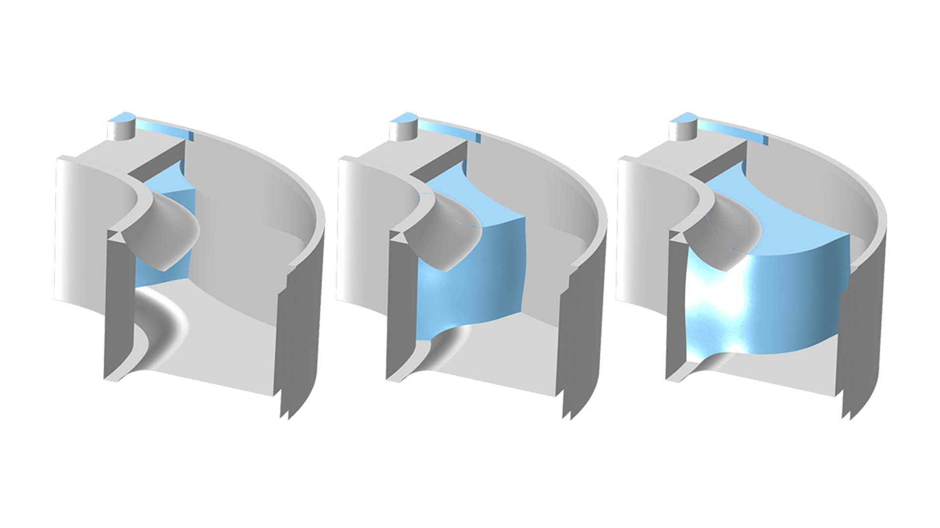
Viscoelastic fluid models account for the elasticity in these types of fluids. As the fluid is deformed, there is a certain amount of force that works toward returning the fluid to its undeformed state. When modeling, it is important to estimate the deformation of the fluid with time (that is, the shape of the air–liquid interface), the local forces on the surfaces that may interact with these fluids, and the pressure losses in a system where the fluid flow occurs. Typical examples of these fluids are polymer melts, paints, and suspensions of proteins.

Colloidal Suspensions, Ketchup, and Lotions

Colloidal suspensions may exhibit shear thickening behavior, where viscosity increases substantially with shear rate. Other suspensions may be shear thinning, for example syrups and ketchup, where the viscosity decreases with shear rate. Thixotropic fluids also have a time dependency, where the viscosity decreases with the duration of the shear rate. The models describing these fluids are all inelastic, but they describe highly non-Newtonian behavior.

The purpose of modeling and simulation is similar to that for viscoelastic fluids above: estimate the shape of the air–liquid interface, the local forces on the surfaces that may interact with these fluids, and the pressure losses in a system where the fluid flow occurs. Additionally, the dependency on temperature and composition may be important for the design of manufacturing processes, such as with the curing of rubber melts, for example.

A mold model shown three times with increasing amounts of blue rubber inside, going from least to most, left to right.

Features and Functionality in the Polymer Flow Module

The Polymer Flow Module offers specialized functionality for many fluid models and properties.

A closeup view of the Fluid Properties settings with the Material model list expanded and Oldroyd-B selected, and an aortic aneurysm model in the Graphics window.

Viscoelastic Fluid Models

The Polymer Flow Module features a variety of viscoelastic fluid models. These models differ in the constitutive relations describing the deformation and the forces caused by the fluid's deformation. The Oldroyd-B model uses a linear relation, which can be described as a suspension of Hookean springs in a Newtonian solvent, while the others describe nonlinear elastic effects and shear thinning.

Oldroyd-B
Giesekus
FENE-P
FENE-CR
Linear Phan-Thien–Tanner (LPTT)
Exponential Phan-Thien–Tanner (EPTT)
Rolie–Poly

A closeup view of the Model Builder with the Two-Phase Flow, Phase Field node highlighted and a slot die coating model at 0.1 seconds in the Graphics window.

Multiphase Flow Models

To make it possible to model the liquid–air interface when simulating coatings, free surfaces, and mold filling, the Polymer Flow Module includes three different separated multiphase flow models based on surface tracking methods. The Level Set method tracks the interface position by solving a transport equation for the level-set function. The Phase Field method tracks the interface position by solving a transport equation for the phase field variable and an equation for the mixing energy density. The Moving Mesh method tracks the interface position with a mesh that changes shape.

A close-up view of the Curing Reaction Heating settings and a basin model in the Graphics window.

Curing in Solids and Liquids

Curing of materials such as composites and adhesives, for which thermal effects are critical to product performance, can be modeled for both fluid and solid domains. With the Curing Reaction interface, temperature-dependent cure kinetics can be defined to represent the chemical curing process. This interface supports various reaction models, including the Sestak–Berggren, Kamal–Sourour, and nth-order models, as well as viscosity models such as the Castro–Macosko and percolation models, enabling accurate prediction of material behavior during the curing process.

A closeup view of the Fluid Properties settings with the Inelastic model list expanded and Power law selected, and a non-Newtonian fluid mixer in the Graphics window.

Inelastic Non-Newtonian Models

In addition to the viscoelastic models, the Polymer Flow Module features a wide range of inelastic non-Newtonian models. Many of the models are generic and used for describing shear thinning and shear thickening. For more specific applications, there are models for viscoplastic and thixotropic fluids.

Power law
Carreau
Carreau–Yasuda
Cross
Cross–Williamson
Sisko
Ellis
Bingham–Papanastasiou (Viscoplastic)
Casson–Papanastasiou (Viscoplastic)
Herschel–Bulkley–Papanastasiou
Robertson–Stiff–Papanastasiou
DeKee–Turcotte–Papanastasiou
Houska thixotropy (Thixotropic)

A close-up view of the Thermal function list expanded and an internal mixer model in the Graphics window.

Thermal Functions for Temperature Dependence

A common method of polymer extrusion and mold filling is to melt the rubber or polymer mixture. The mixture is then allowed to cure inside the mold. The Polymer Flow Module includes the thermal models required to model these processes: the Arrhenius, Williams–Landel–Ferry, and Exponential models are all available.

A close-up view of the Model Builder with the Porous Medium node highlighted and an artery model in the Graphics window.

Porous Media Flow

The Polymer Flow Module enables modeling of non-Newtonian flow in porous media using Darcy and Brinkman formulations for coupled free and porous domains. It includes the following inelastic, shear-dependent viscosity models:

Power law
Carreau
Carreau–Yasuda
Cross
Cross–Williamson
Sisko

Polymer Flow Module

Polymer Melts, Paints, and Protein Suspensions

Colloidal Suspensions, Ketchup, and Lotions